. Introduction
Freshwaters are experiencing significantly greater biodiversity loss than terrestrial ecosystems (Dudgeon et al., 2006). Factors causing freshwater biodiversity declines are linked mainly to human activities. Agriculture, deforestation, and industrial activities throughout entire catchments and river basins influence changes in the water regime and trophic conditions, leading to the destruction of aquatic habitats (Vaughn, 2010). Therefore, freshwater habitats, including lakes, rivers, and wetlands worldwide, continue to face water abstraction, fragmentation, pollution, and damage. Fragmentation and ongoing, negative changes in habitats can strongly affect the genetic diversity of plants, resulting in reduced genetic diversity in dwindling populations (Aguilar et al., 2019). Low genetic diversity can have adverse consequences for fitness and may limit the ability to respond to ongoing environmental changes (Baguette et al., 2012).
Consequently, effective conservation planning requires not only information about species’ biology and ecology but also about the levels and distribution of genetic diversity across their range (Kahilainen et al., 2014). It is usually impossible to conserve all natural populations, especially of rare but widely distributed species. Therefore, efforts must be focused on selected populations or individuals that contribute the most to the existing genetic variation. Recognizing genetic diversity and its spatial structure is crucial to indicate which populations or individuals are particularly valuable for conservation purposes. The question arises of whether it is more important to preserve the largest number of populations across the range or, in cases with a higher level of variation within populations than among them if it is sufficient to retain fewer populations but with a higher number of individuals per locality.
The analysis of spatial genetic structure allows us to determine whether geographically peripheral populations are genetically different from core populations and whether it is essential to prioritize conservation efforts on populations located on the edge of the species’ overall distributional range (Millar & Libby, 1991). Peripheral populations, due to marginal ecological conditions, can experience more rapid cycles of extinction and recolonization associated with the founder effect or population bottlenecks. Consequently, within-population diversity can be low, but genetic variation between core and peripheral populations, or among different, small, and isolated peripheral populations, can be very high (Eckert et al., 2008). The adaptive potential of peripheral populations and their ability to cope with environmental changes can be especially important in the context of climate change (Peterson et al., 2018; Rehm et al., 2015).
The focus of this study is Potamogeton rutilus Wolfg. (Potamogetonaceae), a freshwater plant found mainly in northern Europe, with scattered localities in Asia (Bobrov et al., 2018). In Europe, it has been documented in several countries, including Great Britain (Scotland), Denmark, Norway, Sweden, Finland, France, Germany, Poland, the Baltic countries, Belarus, Ukraine, and European Russia (Hagström, 1916; Hämet-Ahti et al., 1998; Kravchenko, 2009; Lisitsyna et al., 2009; Mäemets, 2016; Preston & Croft, 1997; Tzvelev, 2000; Zalewska-Gałosz, 2008).
Throughout its range, P. rutilus occurs only locally and is regarded as the rarest Potamogeton species (Preston & Croft, 1997). Over the last century, P. rutilus has declined in many of its former localities in Europe, including France, Scotland (Wallace, 2005), Germany, and Poland. Due to the significant loss of populations, P. rutilus is regarded as Critically Endangered in Germany (Metzing et al., 2018), Poland (Zalewska-Gałosz & Pliszko, 2014), and Denmark (Hartvig et al., 2015). It is categorized as Endangered in Estonia (Mäemets, 2016), Vulnerable in Sweden (SLU Artdatabanken, 2020) and in parts of Russia (Bobrov et al., 2018), and Near Threatened in Norway (Solstad et al., 2021), Finland (The red list of Finnish species, 2019; http://hdl.handle.net/10138/299501) and Great Britain (Raper, 2023).
The aim of this study is to assess the distribution of molecular variation and genetic structure within P. rutilus populations across a geographical gradient (Figure 1). Using high-resolution AFLP genotyping (Vos et al., 1995), we addressed three specific questions: (1) Does genetic structure vary within P. rutilus populations? (2) Is there a correlation between genetic diversity and geographic distance among populations? (3) Is the small, peripheral population in Poland, located at the southern edge of the current P. rutilus distribution, genetically distinct from core populations? Based on the results, we aimed to formulate recommendations for the management and conservation of P. rutilus resources.
Figure 1
Map of the sampled populations of Potamogeton rutilus Wolfg. Abbreviations of population codes are explained in Table 1. The dashed red line indicates the likely general area where scattered localities of P. rutilus are distributed. Based on Zalewska-Gałosz and Pliszko (2014) and Bobrov et al. (2018).
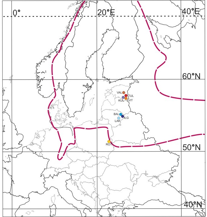
Table 1
Origin of the plant material and parameters of genetic diversity for populations of Potamogeton rutilus in the present study. Abbreviations: Code – code of population; Ni – number of individuals sampled in each population proportional to population size; Ng – number of unique genotypes within samples; NB – number of bands; PB% – percentage of polymorphic bands; IB – number of private bands in population; LCB – number of locally common bands; h – Nei’s genetic diversity mean ± SD; I – Shannon’s information index mean ± SD.
. Materials and methods
. Study species
Potamogeton rutilus belongs to the section Graminifolii, which comprises linear-leaved pondweeds (Preston, 1995). The species is morphologically well-defined and easily identifiable in the field. P. rutilus is an annual that typically reproduces vegetatively through turions or generatively by seeds. The plants have several-flowered spikes projecting above the water surface, which facilitate wind pollination. Members of the section Graminifolii produce bisexual flowers able for self-fertilization (Kaplan & Štěpánek, 2003). Except for anemogamy, also autogamy, hydrogamy, and geitonogamy were evidenced in the group. Turions are produced in late summer and serve to carry the colony over the winter since the rest of the plant dies down. Propagules are dispersed by water (hydrochory) or waterfowl (zoochory). The chromosome number for this species is 2n = 26 (Kaplan et al., 2013). In Europe, P. rutilus thrives in unpolluted, lowland environments, primarily in mesotrophic waters, occasionally in oligotrophic or eutrophic standing waters, alkaline or those that receive some level of base-enrichment, typically on sandy or silt-sandy bottoms (Bobrov et al., 2018; Wallace, 2005).
. Plant material
For our study, we collected samples of P. rutilus growing in three countries: Poland, Lithuania, and Estonia. The studied populations naturally formed three geographical clusters corresponding to the sampled countries. Populations in Estonia and Lithuania occur more within the center of the P. rutilus range, while the population in Poland, in the lake Rotcze (Łęczyńsko-Włodawskie Lake District), is situated at the southernmost extent to the current P. rutilus distribution (Figure 1). The lake Rotcze covers an area of 45 hectares with an average depth of three meters. The lakebed consists of sand, and most of its shores are marshy. The population of P. rutilus thrives in the southeastern part of the lake, near the recreational beach. The lake is not subject to any form of nature protection. The primary threat to this population is the overgrowth by larger macrophytes found in the lake, such as Stuckenia pectinata or Myriophyllum spicatum. We analyzed eight populations, with approximately 10 individuals per population used for the AFLP analysis, resulting in a total of 76 individuals. Detailed list of localities is provided in Table 1. Reference herbarium specimens were prepared for DNA samples and have been deposited in the Herbarium of the Institute of Botany, Jagiellonian University, Krakow (KRA).
. DNA extraction and Amplified Fragment Length Polymorphism (AFLP) fingerprinting analysis
Samples were collected in a field from individuals of P. rutilus at a distance of at least two meters from each other. Each sample consisted of fresh leaves, which were stored in plastic tubes with silica gel and preserved at room temperature till DNA isolation. Total DNA was extracted from ca. 10 mg of dried plant material using Mixer Mill 300 (Retsch) and the DNeasy Plant Mini Kit (Qiagen) according to the manufacturer’s protocol (the final elution step was carried out using 2 × 50 µL elution buffer). DNA quality and concentration were estimated against λ-DNA on 1% agarose gel stained with ethidium bromide.
AFLP fingerprinting analysis followed the procedure of Vos et al. (1995) with modifications as described in detail by Ronikier et al. (2008). Double-digestion of DNA was performed using EcoRI and MseI enzymes. Subsequently, double-stranded EcoRI/MseI adapters were ligated to the digested DNA using T4 DNA ligase. Polymerase chain reaction (PCR) amplifications were performed on a GeneAmp 9700 thermal cycler (Applied Biosystems). Preselective PCR used EcoRI-A and MseI-C primers. Subsequently, selective PCR reactions were performed using 5′-fluorescence-labeled EcoRI selective primers (6-FAM). Selective amplification products were separated using 36 cm capillaries and POP 4 polymer (Applied Biosystems) with Genescan ROX-500 (Applied Biosystems) internal size standard on an ABI PRISM 3100-Avant automated sequencer (Applied Biosystems). At the preliminary screening step, 12 selective primer pair combinations were tested and evaluated for clarity of profiles (i.e., prevalence of well-separated markers) and number and repeatability of polymorphic markers. Three primer pairs were selected for the final analysis: Eco-ACC/Mse-CAG, Eco-ACA/Mse-CAT, and Eco-AGA/ Mse-CTG. AFLP fragments were manually scored using Genographer 2.1 (http://sourceforge.net/projects/genographer). The reproducibility of AFLP markers was assessed using 12 within-plate and four between-plate sample replicates (based on single DNA extractions) carried in parallel through all reaction steps. The error rate was calculated as the percentage of mismatches in the scoring of AFLP profiles of replicated individuals. Only markers that scored unambiguously (i.e. were well separated) and repeatedly in the duplicates were considered. AFLP fragments in the size range of 50–500 bp were scored and assembled in a binary presence/absence matrix.
. Molecular variation and genetic structure
Genetic variation within populations was determined as the percentage of polymorphic bands (PB%), the number of private bands (IB; occurring in all the individuals in a defined group and completely absent in other samples), and the number of locally common bands (LCB; occurring in 50% of populations or fewer with frequency >= 5%). The level of genetic variation was determined based on Nei’s gene diversity (h; Nei, 1978) and Shannon’s information index (I; Brown & Weir, 1983), calculated in GenAlEx 6.5 software (Peakall & Smouse, 2006). The Kruskal–Wallis H tests, followed by Dunn’s post hoc tests, were used to test the differences in genetic diversity parameters (i.e., Nei’s gene diversity (h) and Shannon’s information (I) indexes) between studied populations. The analysis was performed using Statistica 13 (StatSoft, Tulsa, OK).
The overall genetic relationships among studied individuals were explored using the principal coordinate analysis (PCoA) based on Nei’s genetic distances (Nei, 1978). The cluster analysis was performed on the unweighted pair-group method using arithmetic means (UPGMA) and the Jaccard similarity coefficient to visualize genetic diversity derived from AFLP markers of particular individuals and to detect putative clones and individuals created by selfing mode of reproduction, with high levels of AFLP profile similarity. The analysis was done using PAST 3.25 (Hammer et al., 2001).
The analysis of molecular variance (AMOVA) was based on groups defined a priori (populations) by separate water bodies (lakes). AMOVA was based on the pairwise squared Euclidean distance among molecular phenotypes. Significance levels were determined by 999 permutations. AMOVA and PhiPT index and gene flow (Nm) were calculated using GenAlEx 6.5 software.
The most likely number of population clusters was estimated in the STRUCTURE 2.3.2 software (Pritchard et al., 2000), with the model for dominant markers (Falush et al., 2007), correlated allele frequencies, and admixture. STRUCTURE uses a Bayesian clustering algorithm to assign individuals to a specified number of clusters (K value). Additionally, as the method might be sensitive to the number of individuals sampled in each population (Puechmaille, 2016), we explored a range of program parameters, with the alpha parameter 0.25 and: (a) allelic frequencies uncorrelated among populations; (b) allelic frequencies correlated with populations; (c) separate estimations of alpha parameter for each population and allelic frequencies uncorrelated among populations, as suggested by Wang (2017). Each analysis was run with 200,000 burn-in cycles and 1,000,000 sampling MCMC cycles, for K value between 1 and 8 (eight populations analyzed in the study), in five replicates each. CLUMPAK (Kopelman et al., 2015) was used to determine the optimal K value using the ΔK method (Evanno et al., 2005) and to align all optimum K STRUCTURE runs to the permutation with the highest H-value and visualize the output.
For reconstructing the relationships among the studied populations and identifying population clusters, the NeighbourNet analysis was used with uncorrected p-distances, as implemented in Splits-Tree4 version 4.11.3 (Huson & Bryant, 2006). Bootstrap support for splits was calculated using 1000 replicates (Felsenstein, 1985).
The Mantel test (Mantel, 1967) with 9999 random permutations was performed to determine the relationship and statistical correlation between the two matrices of distance, i.e. the genetic distance matrix (Nei’s genetic distances) and the geographical distance matrix. Euclidean coefficients were applied to both matrices. This was done in order to determine whether between-populations similarities in terms of genetic distance and geographical distance were significantly interrelated. The analysis was done using PAST 3.25 (Hammer et al., 2001).
. Results
. Genetic structure
AFLP fingerprinting of P. rutilus yielded high-quality profiles, with marker reproducibility averaging 96.05%, based on the evaluation of duplicated profiles. We analyzed a total of 76 individuals from eight P. rutilus populations. Three selective primer combinations produced 184 high-quality markers. The total number of polymorphic markers was 88. Specifically, the percentage of polymorphic bands in each population ranged from 21.74% (TUL, Estonia) to 0% (LAK, Lithuania), with an average of 11.07% polymorphic bands. The number of private bands varied from 0 (LAK, Lithuania, and VAL, Estonia) to 11 (TUL, Estonia).
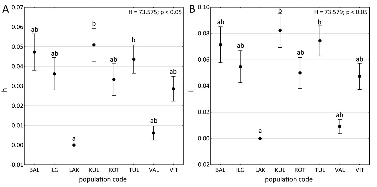
Nei’s gene diversity ranged from 0.000 (LAK, Estonia) to 0.051 (KUL, Estonia), with a population mean of 0.031 (SD = 0.003). Similarly, Shannon’s information index ranged from 0.000 (LAK, Estonia) to 0.082 (KUL, Estonia) with a population mean of 0.049 (SD = 0.004) (Table 1). Notably, population LAK exhibited significantly lower Nei’s gene diversity and Shannon’s information index compared to population KUL and TUL (Kruskal–Wallis H test; p < 0.05, Figure 2).
Figure 2
Box-and-whisker plots of genetic diversity parameters for particular populations of Potamogeton rutilus. (A) mean ± SD Nei’s gene diversity (h); (B) mean ± SD Shannon’s information index (I). Points indicate mean values, whiskers indicate standard errors. Results of Kruskal–Wallis H tests (p < 0.05): H and p values are provided. Letters denote the results of Dunn’s post hoc tests; different letters indicate significant differences at the p < 0.05 level. Abbreviations of population codes are explained in Table 1.
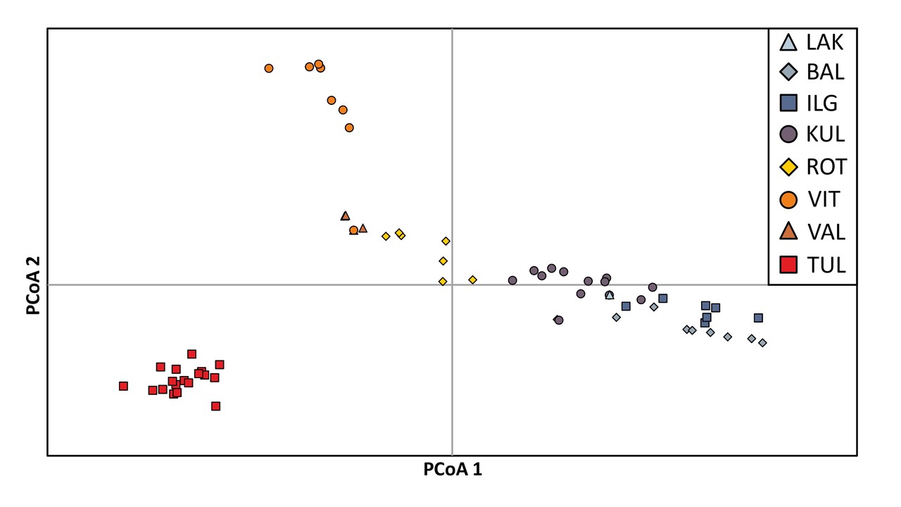
The Principal Coordinates Analysis (PCoA) revealed distinct genetic differentiation of studied individuals along the first axis, which accounted for 22.91% of the observed variation in P. rutilus (see Figure 3). The individuals from populations from Lithuania (BAL, IGL, and LAK) and one from Estonia (KUL) were separated from individuals from the remaining Estonian populations (VIT, VAL, TUL). Individuals from population located in Poland (ROT) are placed between these two groups, indicating their genetic similarity to both these genetic groups. The PCoA diagram also highlighted the unique position of Estonian populations TUL and VIT along the second axis, accounting for 16.37% of the observed variation.
Figure 3
Principal coordinate analysis (PCoA) of AFLP data based on Nei’s genetic distances for individuals representing particular populations of Potamogeton rutilus. Abbreviations of population codes are explained in Table 1.
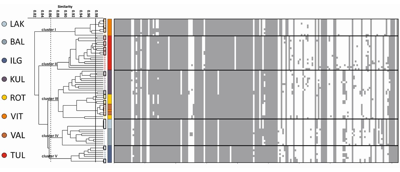
Cluster analysis based on individual data identified five primary clusters at a similarity level of 86% (see Figure 4). Cluster I represents the most isolated group, consisting solely of individuals from the Estonian VIT population. Cluster II comprises all individuals from the Estonian TUL population. Clusters IV and V exclusively consist of individuals originating from Lithuanian populations, with cluster IV containing individuals from the LAK and BAL populations and cluster V including only those from the ILG population. Cluster III proved to be the most diverse in terms of individual origin. Within this cluster, we observed a division into two subclusters, A and B, sharing a similarity of 88%. Subcluster A encompasses individuals from the Estonian KUL population, while subcluster B includes individuals from both Poland (ROT) and Estonia (VIT, VAL). The UPGMA dendrogram revealed putative clones or individuals created by selfing mode of reproduction, that were characterized by more than 98% genetic similarity (Figure 4 marked with black squares). In each population, except for BAL, such individuals were present. Altogether, 52 AFLP profiles out of 76 studied individuals are unique; the most genetically diverse is population TUL (Table 1, Figure 4) shared identical or very similar profiles, i.e., one or two band differences.
Figure 4
The results of cluster analysis performed on the unweighted pair-group method using arithmetic means (UPGMA) using the Jaccard similarity coefficient presenting genetic diversity based on AFLP profiles of Potamogeton rutilus. On the right side, AFLP profiles for particular individuals are provided. All samples separated at a level higher than 98% similarity can be considered as putative clones or individuals created by selfing mode of reproduction, and are marked with black squares. Abbreviations of population codes are explained in Table 1.
In an analysis of molecular variance (AMOVA), 63% of the total genetic variation was among populations, while 37% was within populations (PhiPT = 0.634, p < 0.001; see Table 2). The overall rate of gene flow (Nm) throughout the entire sampled area based on the PhiPT equaled 0.289. The gene flow (Nm) varied from 0.026 to 0.757 between eight studied populations. The highest value was recorded between KUL and ROT populations, whereas the lowest was between VIT and LAK (Table 3).
Table 2
Analysis of molecular variance (AMOVA) based on AFLP markers for eight populations of Potamogeton rutilus. Abbreviations: df – degrees of freedom; SS – sum of squares; MS – mean square; Est. var. – estimated variance; Per. var. – percentage of variation; Nm – gene flow based on the PhiPT.
| Variation | df | SS | MS | Est. var. | Per. var. | PhiPT | p | Nm |
|---|---|---|---|---|---|---|---|---|
| Among populations | 7 | 442.995 | 63.285 | 6.438 | 63% | |||
| Within populations | 68 | 252.742 | 3.717 | 3.717 | 37% | |||
| Total | 75 | 695.737 | 10.155 | 100% | 0.634 | 0.001 | 0.289 |
Table 3
Genetic differentiation and gene flow between different populations. The lower triangle represents the genetic differentiation coefficient (PhiPT), and the upper triangle represents gene flow (Nm) between populations.
An isolation-by-distance analysis using the Mantel test did not reveal a significant correlation between genetic distance and geographical distance among populations (R = −0.05; p = 0.56; Figure S1).
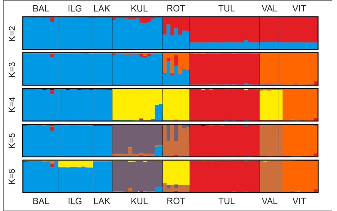
In the STRUCTURE analysis of AFLP data, the highest log-likelihood value (Pritchard et al., 2000) was found for K = 6 (Figure S2A), but the optimal number of population groups (K) according to Evanno et al. (2005) was four (Figure S2B). The first division (K = 2) was formed between Lithuanian populations (ILG, BAL, and LAK), including one population from Estonia (KUL), and the rest of Estonian populations (TUL, VAL, VIT), including population from Poland (ROT). For K = 3, the third group was formed by the Estonian population TUL. For K = 4, the Lithuanian populations IGL, BAL, and LAK were still separated from two Estonian populations, KUL and VAL, which were grouped together with the Polish population ROT. Additionally, two new groups were built by Estonian populations, TUL and VIT. For K > 4 ≤ 8, in the majority of runs, Lithuanian populations ILG, BAL, and LAK formed one group, while each of the other populations was divided as separate groups with different portions of admixture within the groups. For K ≥ 4, one individual from the VIT population is shown as genetically identical to individuals from the VAL population and clearly distinct from the rest of individuals from its native population VIT (Figure 5).
Figure 5
Results of Bayesian analysis using STRUCTURE with the model for dominant markers, constant alpha = 1, correlated allele frequencies and admixture. Bar graphs of individuals for K = 2–6; populations are separated by vertical lines. Population codes are explained in Table 1.
In the model with alpha = 0.25 and allelic frequencies correlated among populations, our STRUCTURE results mirrored those described for alpha = 1 (Figure S3). In the model with alpha = 0.25 and allelic frequencies uncorrelated among populations, the optimal K value according to the Evanno method was two, but the highest log-likelihood value was found for K = 5. For K = 2, in this model, the Estonian population TUL was separated from the rest populations in the study. For K = 5, five groups were formed: Lithuanian (populations BAL, LAK), Estonian, made by populations KUL and VAL with the one Polish population ROT, and three separate groups each of them formed by one population: IGL, TUL, and VIT. For the model with separate alpha parameter estimation for each population and allelic frequencies uncorrelated among populations, the optimal population group was K = 3 according to the Evanno method. For this value, Lithuanian populations (ILG, BAL, and LAK) and one population from Estonia (KUL) formed one group, another group comprised Estonian populations (VAL, VIT) together with the Polish population ROT while the Estonian population TUL formed a separate, third group. In this model, the highest log-likelihood value (Pritchard et al., 2000) was found for K = 6. For this value, the separate position of the Estonian population TUL was still maintained. Populations KUL, ROT, and VAL formed the second group; however, populations ROT and VAL showed some affinities to population VIT, which formed the next, separate group. The fourth group was composed of Lithuanian populations BAL and LAK, and the fifth group included the Lithuanian population IGL, showing some similarities with both Lithuanian populations BAL and LAK (Figure S4).
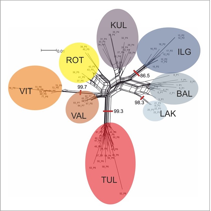
NeighbourNet analysis unveiled that the studied populations of P. rutilus can be categorized into five main clusters (see Figure 6). The first cluster consists of the Estonian population TUL, the second cluster encompasses two Estonian populations, VAL and VIT, the third cluster comprises the Polish population ROT, the next cluster is formed by the Estonian population KUL, and the final cluster comprises Lithuanian populations LAK, BAL, and IGL.
Figure 6
NeighbourNet analysis of the amplified fragment length polymorphism (AFLP) dataset of Potamogeton rutilus populations. Shaded ovals indicate populations, their codes are explained in Table 1.
. Discussion
Despite of discrete, island-like distribution of aquatic habitats, freshwater macrophytes show broader distributional ranges in comparison to terrestrial plants (Santamaría, 2002; Sculthorpe, 1967). Land plant distribution is often limited by climatic conditions, while aquatic environments, owing to their natural buffering capacity provided by water, tend to be more stable and resistant to temperature fluctuations and other climatic variables. However, even within water bodies on a small geographic scale, aquatic habitats can vary significantly in factors such as light, temperature, oxygen levels, and nutrient concentration. This variability in ecological conditions among neighboring aquatic habitats can render them more isolated than would be expected based solely on geographic distance. Given these considerations, although understanding genetic structure is crucial for effective species conservation planning, predicting the distribution of genetic variation is impossible without detailed genetic research.
Our study results indicate that the genetic variation of P. rutilus in mainland Europe, excluding Scandinavia, is relatively low. This variation is primarily generated by the variation among populations (63%) rather than within them (37%). This finding aligns with the previously observed pattern of genetic variation distribution in macrophytes, including Potamogeton (e.g. Hardion et al., 2021; Hettiarachchi & Triest, 1991; Hollingsworth et al., 1995; Iida & Kadono, 2002; Kaplan & Štěpánek, 2003; Philbrick & Les, 1996), as well for P. rutilus directly (Wallace, 2005). Such variation distribution can be attributed to the founder effect, limited seedling recruitment, and the prevalence of clonal propagation. Vegetative reproduction is both rapid and efficient in aquatic environments. Specialized and non-specialized propagules alike can reduce the risk of genotype mortality (Barrett et al., 1993; Philbrick & Les, 1996; Zalewska-Gałosz & Ronikier, 2010). The effectiveness of vegetative propagation is particularly well-documented in the case of sterile Potamogeton hybrids, which can persist within one locality for centuries (e.g. Kaplan & Fehrer, 2007; Zalewska-Gałosz, 2010; Zalewska-Gałosz et al., 2018). In our study, ca. 50% of individuals are putative clones characterized by identical or very similar AFLP profiles (i.e., one or two band differences, which corresponds to up to 2% genetic dissimilarity). Amplified fragment length polymorphism has been commonly used for clone identification, and most studies reported threshold genetic dissimilarity distance between 2% and 4% below which samples are considered to represent a single clone (e.g., Douhovnikoff & Dodd, 2003; Lasso, 2008).
Despite a significant prevalence of clonal reproduction, the observed genetic variability, as indicated by the percentage of polymorphic bands in populations, suggests the presence of generative reproduction. This is particularly evident in Estonian populations KUL and TUL, as well as in Lithuanian populations ILG and BAL. Both modes of reproduction realized by P. rutilus were also confirmed by Wallace (2005) through RAPD analysis of genotype variation in six lochs in Scotland. Moreover, Wallace (2005) detected significant differences in the distribution of genotypic diversity between adjacent water bodies and suggested a trend where genetic diversity increases as P. rutilus population size decreases. This observation could reflect reduced success in vegetative reproduction in potentially unfavorable environments, with sexual reproduction favored in more stressful environmental conditions (Sculthorpe, 1967). However, this trend is not observed in our study, where the most genetically diverse are relatively large Estonian populations TUL and KUL, while the small population in Lithuania, in Lake Lakajai (LAK), clearly represents a single clone (Table 1, Figure 4). The lack of a consistent and clear pattern of distribution of genetic variation reflects the diversity of factors influencing the formation of genetic variation within and among populations of P. rutilus. These factors include not only the mode of reproduction but also the number of founding individuals, population age, size, and niche differentiation.
Our study revealed a marked genetic structure of P. rutilus populations. According to NeighborNet, principal component analysis (PCoA), and the STRUCTURE analyses, regardless of the parameters used, the studied populations clustered into three main genetic groups that align with their geographic distribution, specifically Lithuanian (BAL, ILG, LAK) and Estonian (VIT, TUL). However, Estonian populations TUL and VIT displayed their own distinctiveness and constituted separate groups. Populations ROT, VAL, and KUL exhibited genetic affinities that did not align with their geographic distribution. The revealed high differentiation among populations of P. rutilus may be explained by the limited number of effective migrants (Nm = 0.289). The gene flow varied from 0.026 to 0.757 within eight populations in our study. The exchanges of migrants can be facilitated by the relatively short distance between Lithuanian populations LAK and ILG (Nm = 0.165) as well as between Estonian populations VIT and VAL (Nm = 0.388), in which we detected relatively low gene flow. More surprising and difficult to explain is the genetic similarity of the ROT population, located at the southern edge of the P. rutilus range, to the Estonian populations VAL and VIT, rather than to the geographically closer Lithuanian populations: ILG, BAL, or LAK. In the case of aquatic plants, waterfowl serve as excellent vectors for transporting seeds over long distances (Barrett et al., 1993; Lukács et al., 2020). Although, aside from ROT, the Estonian population KUL also shows higher genetically similarity to Lithuanian populations than the rest of the Estonian ones, which does not align with geographic distance (Figure S1), it is more plausible that the genetic structure revealed by our study reflects an ancient pattern of genetic variation shaped by successive extinction and re-colonization events, which is difficult to understand based on the limited sampling of the present-day study.
In Scotland and mainland Europe, excluding Scandinavia, P. rutilus is classified as oligo-mesotrophic. Therefore, the disappearance of this species is at least partially correlated with anthropopression, pollution, eutrophication, and increased salinity (e.g. Mäemets, 2016; Preston & Croft, 1997; Wallace, 2005). One of the factors threatening plant species can be interspecific hybridization (Ottenburghs, 2021; Zalewska-Gałosz et al., 2023). While hybridization between P. rutilus and P. friesii has indeed been confirmed, it occurs extremely rarely (Zalewska-Gałosz & Ronikier, 2011). Therefore, in the case of P. rutilus, this threat should be considered as irrelevant.
The decline of P. rutilus populations in mainland Europe may be accelerated by ongoing global warming, leading to the eutrophication of freshwaters. However, the threat doesn’t solely arise from eutrophication itself, as P. rutilus can form persistent populations also in eutrophic, cold waters in Scandinavia (Virola et al., 2001). Instead, it primarily results from the competitive growth of more robust aquatic plants, which is encouraged by nutrient-rich conditions and higher water temperatures.
Our study unequivocally shows that in mainland Europe P. rutilus is genetically coherent and does not encompass highly divergent genetic lineages. Our data indicates that the small and peripheral population ROT in Poland, which is intuitively considered a special conservation value, is generically similar to the Estonian populations VIT and VAL. We did not identify unique gene pools that would warrant special protection for this population. However, our research revealed that each studied population possesses specific genetic characteristics due to the spatial isolation in separate lakes and very limited gene flow. Therefore, management efforts should focus on maintaining as many populations as possible and actively protecting P. rutilus by preventing overgrowth from larger macrophytes, thereby averting the loss of genetic diversity due to genetic drift. Further research should concentrate on the local adaptation of P. rutilus populations to ongoing ecological and climatic changes by employing niche modeling and identifying both neutral and adaptive genetic variations. Furthermore, for conservation purposes, it’s intriguing to recognize the genomic basis of the success of P. rutilus in Finland, where this species effectively colonizes new sites in eutrophic lakes and expands its range (Virola et al., 2001).
. Supplementary material
The following supplementary materials are available for this article:
Figure S1. Nei’s genetic distance as a function of geographic distance for studied populations of Potamogeton rutilus. The coefficient of correlation between geographic and genetic distance was calculated using a Mantel test.
Figure S2. Detection of the number of groups (K) in STRUCTURE analyses of the AFLP datasets for Potamogeton rutilus. The graphs show (A) the mean value of log probability of the data; L(K), as a function of K ranging from 1 to 8 as estimated by the program STRUCTURE, and (B) the rate of change in the probability between successive runs; Delta K, as a function of K, calculated according to Evanno et al. (2005).
Figure S3. Results of Bayesian analysis using STRUCTURE with the model for dominant markers, constant alpha = 0.25, and allelic frequencies correlated among populations. Bar graphs of individuals for K = 2–6; populations are separated by vertical lines, and their codes are explained in Table 1.
Figure S4. Results of Bayesian analysis using STRUCTURE with the model for dominant markers, with separate alpha parameter estimated for each population and allelic frequencies uncorrelated among populations. Bar graphs of individuals for K = 2–6; populations are separated by vertical lines, and their codes are explained in Table 1.