. Introduction
The health status of forests on a global scale has changed considerably because of the acceleration of climate change and collapse of ecosystems (Curtis et al., 2018; Thomas et al., 2004). The protection and restoration of forests is crucial for the mitigation of global climate change and biodiversity conservation (Chiarucci & Piovesan, 2019). Issues arise when considering how to monitor forest dynamics, measure the health status of forest ecosystems, and in determine the extent of human impact. Biodiversity has been viewed as a quantitative characteristic that can be assessed or measured by a number of direct indices reflecting the overall holistic characteristics of biodiversity (Feest, 2013), here described as “biodiversity quality” (Feest, 2006).
A recent study by Ambrosio et al. (2018) and Feest (2013) showed that relevant information regarding biodiversity may be extrapolated through organisms that are indicators of ecosystem functions and conditions. This aspect is particularly important given the need for the development of methodologies that would reduce the time and costs involved in biological conservation and monitoring actions (United Nations, 2017).
In this sense, fungal biodiversity can potentially provide an indication of ecosystem changes because it is closely related to overall site biodiversity and expresses the heterogeneity of a habitat (Boddy et al., 2014; Büntgen et al., 2011; Egli, 2011; Kauserud et al., 2008, 2010; Kotiranta & Niemelä, 1993). Several studies have confirmed that changes in fungal communities may reflect the degree of forest degradation (Egli, 2011; Stursova et al., 2014). Hence, monitoring the composition and dynamics of the fungal community over time and space may represent a useful tool for evaluating the health status of forests and establishing conservation priorities in different locations (Egli, 2011; Feest, 2013; Halme & Kotiaho, 2012). Fungi are among the most important organisms on Earth and are essential components of terrestrial ecosystems because of their functional roles and high species richness and diversity (Blackwell, 2011; Hawksworth, 2001; Mueller & Schmit, 2007). They profoundly affect forest ecosystem functions by driving the carbon cycle, decomposing organic matter, mediating nutrient and water uptake, protecting roots from fungal pathogens, and maintaining soil structure and forest food webs (Heilmann-Clausen et al., 2014; Tedersoo et al., 2014). Moreover, the fungal reproductive (and ephemeral) structures (viz. fruiting bodies/sporocarps) are strictly dependent and affected by climatic (e.g., light, microclimate, rainfall) and edaphic conditions (e.g., pH, nutritional factors, organic matter) (Boddy et al., 2014). In vitro growth experiments have shown that climate variables (e.g., rising temperatures) influence fungal physiology and growth (Boddy et al., 2014); hence, their presence/absence, or community variation over time and space may be used as indirect indicators of climate change and predictors of forest health status and dynamics.
Due to the key role played by fungi in detecting early changes in habitats and environments, e.g., nitrogen deposition as in Baar and Kuyper (1998), Feest et al. (2014), and Mohan et al. (2014), as well as their importance in ecological and conservation studies, the macrofungal biodiversity quality of eight Mediterranean forests located in Italy was investigated using a standardized survey approach (Feest, 2006).
The goals of this study were: (i) to evaluate the influence and relationship of forest types and management on macrofungal biodiversity quality indices; (ii) to identify possible macrofungal species indicators of Mediterranean forests; and (iii) to assess macrofungal biodiversity quality over the years. We postulated the following hypotheses:
Different Mediterranean forests, which differ in vegetation type and management, have statistically different macrofungal biodiversity quality indices.
A site surveyed over consecutive years will have statistically different macrofungal biodiversity quality indices as a result of abiotic factors (e.g., climate variations).
In this study, biodiversity quality is regarded as the quality of a site that can be extrapolated from a number of measured characteristics of the population studied (here macrofungi) that are present at the time of sampling (Ambrosio et al., 2018; Feest, 2006).
. Material and Methods
. Study Sites
Eight sites were selected from northern to southern Italy (including islands) along a latitudinal gradient (Figure 1). These forest types are representative of Mediterranean (Italian) vegetation (Blasi et al., 2007; Mariotti, 2008). Specifically, Site 1 (S1 in figures and tables) is a silver fir plantation (Abies alba Mill.) located in Sardinia; Sites 2 (S2) and 8 (S8) are both chestnut coppices, dominated by Castanea sativa Mill. [lower frequency of other woody species occurs at these sites, such as Sorbus torminalis (L.) Crantz and Populus tremula L.], which are located in Liguria (S2) and Campania (S8), respectively. Both sites (S2 and S8) are subject to human intervention (i.e., by cutting and thinning) to clear the undergrowth vegetation and facilitate the collection of chestnuts. Sites 3 (S3) and 5 (S5) are characterized by deciduous oak (Quercus cerris L.) woods and are managed as high priority forests consisting of large, tall, and mature trees with a closed canopy. A lower frequency of S. torminalis and P. tremula occurred at these sites. They are located in Liguria (S3) and Tuscany (S5), respectively. Site 4 (S4), located in Liguria, is a beech forest, which is dominated by Fagus sylvatica L. (followed by S. torminalis and P. tremula at lower frequencies), and is also managed as a high priority forest. Finally, Sites 6 (S6) and 7 (S7) are evergreen oak (Quercus ilex L.) woods (ascribed to the Mediterranean maquis landscape), located in Tuscany (S6) and Campania (S7), respectively. All the sites are open to public for picking edible mushrooms under regional and national rules, except S2, S3, and S8, where the access is restricted and picking of edible mushrooms is not allowed because they are located on private property. Only Site 1 can be described as a monoculture. More details on the characteristics of the sites are summarized in Table 1.
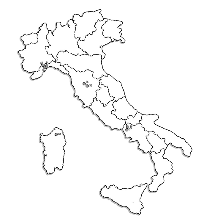
Table 1
Characteristics of study sites.
| Site code | Locality | Coordinates | Altitude (m a.s.l.) | Vegetation | Forest type | Geology | Mean rainfall (mm) | Mean Temperature (°C) | Data references |
|---|---|---|---|---|---|---|---|---|---|
| S1 | Sardegna – Loc. Tempio Pausania (OT) | 40°51′ 7″ N, 9°10′ 13″ E | 1,262 | Silver fir – Abies alba | Unmanaged | Leucogranites rocks | 1,300 | 10 | Ambrosio et al., 2015 |
| S2 | Liguria – Loc. Badani (SV) | 44°27′ 56″ N, 8°28′ 44″ E | 430 | Chestnut coppice – Castanea sativa | Managed | Calceschist rock | 912 | 12 | Ambrosio et al., 2018 |
| S3 | Liguria – Loc. La Maddalena (SV) | 44°30′ 14″ N, 8°29′ 17″ E | 360 | Deciduous oak wood – Quercus cerris | Unmanaged | Serpentine schists | 912 | 12 | Ambrosio et al., 2018 |
| S4 | Liguria – Loc. Veirera (SV) | 44°27′ 3″ N, 8°32′ 42″ E | 1,000 | Beech forest – Fagus sylvatica | Unmanaged | Calceschist rock | 912 | 12 | Ambrosio et al., 2018 |
| S5 | Toscana – Loc. Basciano (SI) | 43°22′ 36.1″ N, 11°17′ 24.9″ E | 328 | Deciduous oak wood – Quercus cerris | Unmanaged | Calcareous soil | 777 | 13.4 | Unpublished data |
| S6 | Toscana – Loc. Montegabbro (SI) | 43°23′ 53.7″ N, 11°02′ 43.7″ E | 297 | Evergreen oak wood – Quercus ilex | Unmanaged | Calcareous soil | 777 | 13.4 | Unpublished data |
| S7 | Campania – Loc. San Felice (CE) | 41°14′ 15.9″ N, 13°58′ 06.8″ E | 210 | Evergreen oak wood – Quercus ilex | Unmanaged | Calcareous soil | 900.8 | 16.1 | Unpublished data |
| S8 | Campania – Loc. Roccamonfina (CE) | 41°18′ 09.5″ N, 13°59′ 12.0″ E | 612 | Chestnut coppice – Castanea sativa | Managed | Vulcanic soil | 925.9 | 15.2 | Unpublished data |
. Survey Procedure
All study sites were surveyed using the same standardized procedure (Feest, 2006). Surveys were performed during the period of maximum sporocarps fruiting and development (in fall, mainly early October in 2013) in 20 circular (4-m radius) plots at each study site along line transects. Each plot was placed 20 m from the preceding plot. The total sample area was approximately 1,000 m2 per site. Sites 2–4 were surveyed over three consecutive years (2012–2014).
Mycological observations were focused on epigeous macrofungi with a determinate shape that were visible to the naked eye, mostly sporocarps (Kirk et al., 2008). Macrofungi were studied both qualitatively (identification of species) and quantitatively (number of sporocarps/fruiting bodies per species). Taxonomical identification was performed by analyzing the macro- and microscopic characteristics of the collected specimens. The systematic classification followed Hibbett et al. (2014) and He et al. (2019). Nomenclature was used in accordance with the Index Fungorum (http://www.indexfungorum.org/), CBS (https://wi.knaw.nl/), and IMA (https://www.mycobank.org/) databases.
. Data Sets
Full datasets are shown in Appendix S1–Appendix S8. To calculate a set of biodiversity indices and statistics (detailed in the next paragraph) for each study site, we defined a dataset as: the total number of fungal species and respective sporocarps/fruiting body abundance. Datasets refer to both published and unpublished data (see Table 1) collected by following the same standardized sampling procedure (Feest, 2006).
. Data Analyses
A set of biodiversity indices (Magurran, 2004), based on the number of individuals (sporocarps/fruiting bodies) collected per study site that were present at the time of sampling, was computed to extrapolate the biodiversity quality (Feest, 2006; Feest et al., 2010) of each selected site, as follows:
Species richness (SR) is the number of species recorded. The SR expresses alpha diversity and is the simplest measure of biodiversity, albeit with low information value.
Population abundance (pA): the number of individuals (sporocarps) for each collected species.
Population density (pd): the total number of individuals recorded in the standardized sample (pd/m2).
Shannon Index (H′) was used to combine the effects of SR and evenness. This index assumes that individuals are randomly sampled, and that all species are represented in the sample. H′ depends on the total number of species and their occurrence.
Pielou Evenness Index (E) was calculated to measure the departure of the observed pattern from the expected pattern in a uniform assemblage of equally abundant species.
Simpson’s Index (D) was computed to calculate the evenness of the population per species. This index is weighted by the abundance of the most common species; when D increases, diversity decreases.
Berger–Parker Index (d) expresses the proportional abundance of the most abundant species.
Nonparametric estimators were used to estimate the SR and to check whether data collected allowed observation of a notable number of species. Specifically, the Chao estimator is the simplest method to extrapolate the predicted number of species in an assemblage, and is based on the number of singleton and doubleton species (Chao, 1984; Magurran, 2004). The first-order jackknife estimator is based on the number of “unique species,” as well as the exact number of species that occur in the sampling units and duplicates, respectively (Heltshe & Forrester, 1983; Magurran, 2004). Finally, the bootstrap estimator for SR was based on the frequency distribution of the species found in the sample (Magurran, 2004; Smith & van Belle, 1984). These estimators indicate the degree of the sampling efficiency.
Rarefaction curves were chosen because they illustrate the rate at which new species are found unless sampling has been exhaustive. The curve generally rises very quickly at first and then flattens once a reasonable number of individuals have been considered (Colwell et al., 2012; Gotelli & Colwell, 2001; Magurran, 2004). In this study, the number of species was plotted as a function of the accumulated number of individuals. We used the function “rarefy” in the VEGAN package version 2.5-7 (Oksanen et al., 2013) to plot the curves with the corresponding iterative error around the mean. Rarefaction generates the expected number of species in a small collection of individuals drawn randomly from the entire pool of individuals. In this study, “individuals” refer to the sporocarps counted and “sample” to plots in each study site.
Species Conservation Value Index (SCVI) (Feest, 2006; Feest et al., 2010) was calculated as the mean commonness/rarity of each species recorded according to national references (Boccardo et al., 2008; Onofri et al., 2005). Accordingly, all species were given a numerical value, as follows: 1 – species occurring in more than 85%–100% of the Italian territory; 2 – species recorded on 65%–85%; 3 – species recorded on 45%–65%; 4 – species recorded on 25%–45%; 5 – species recorded on less than 25% of the Italian territory.
Biomass Index (BI) was estimated using a nondestructive method (Tóth & Feest, 2007). Biomass is directly related to the size of fruiting bodies calculated from the radius of the cap. The BI was computed from the biometrics of the species as dry weight (Feest, 2006).
Indicator species analysis (ISA) (De Cáceres et al., 2010) was used to identify macrofungal indicator species for the selected study sites.
Hierarchical cluster analysis (H-CA) using the Bray–Curtis dissimilarity index and unweighted pair group method with arithmetic mean UPGMA (Legendre & Legendre, 2012) was carried out to discern the degree of similarity between the selected study sites.
Correspondence analysis (CA) was performed to determine the distribution of macrofungal communities without the constraint of biotic and abiotic variables. The variables are represented by species and cases by plots (Legendre & Legendre, 2012).
H-CA and CA were both computed with SR, presence/absence, and Shannon Index obtained in each surveyed plot (160 in total) for all of the selected sites.
The effect of climatic factors (mean temperatures and rainfall) on macrofungal biodiversity indices (SR, pA, H′, and BI) was tested using the multivariate technique of principal correspondence analysis (PCA) (Everitt & Hothorn, 2006). Since the environmental variables were expressed at different measurement scales, PCA was computed on the correlation matrix. Vector fitting was used to identify significant variables on the ordination axes (PCA1 and PCA2).
All statistical analyses were computed using VEGAN and BiodiversityR packages in the R statistical environment (version 4.0.0; 2020).
. Climate Data
Climate data were extracted using the ARPAL database (https://www.arpal.liguria.it/). Specifically, we selected daily data on mean temperature (°C) and mean rainfall (mm) for Sites 2, 3 and 4 (from Loc. Sassello weather station), where we conducted field surveys for three consecutive years (2012, 2013, 2014).
. Results
Overall, mycological surveys were performed in 160 plots for a total sampled area of 8,000 m2. Appendix S1–Appendix S8 list the recorded number of species and sporocarp (mainly basidiomata) abundance collected at each site and plot.
A total of 153 macrofungal species (species richness) were observed in the eight study sites (in 2013): 59 species in the beech forest (S4), 52 species in the silver fir site (S1), 45 and 23 species in the chestnut coppices (S2 and S8, respectively), 35 and 33 species in the evergreen oak woods (S7 and S5), and 34 and 33 species in the deciduous oak woods (S3 and S6, respectively) (see SR column in Table 2).
Table 2
Results of biodiversity indices.
[i] SR – species richness; pA – population abundance; pd – population density; H′– Shannon Index; E – Pielou Evenness Index; D – Simpson’s Index; d – Berger–Parker Index; Chao – nonparametric estimator Chao1; Jack. 1 – jackknife first order – nonparametric estimator; Bood. – bootstrap – nonparametric estimator; SCVI – Species Conservation Value Index; SD – Standard deviation; BI – Biomass Index.
The highest value of population abundance (pA in Table 2) and density (pd) were obtained in the evergreen oak woods (S5; pA = 761, pd = 0.761 m−2), while the lowest was obtained in the beech forest (S4; pA = 162, pd = 0.162 m−2).
The results for the Shannon Index (H′) and Pielou Evenness Index (E) showed very similar values among the sites (Table 2). Specifically, values of H′ ≥ 3 were computed for Sites 1–4 and Site 7; in contrast, values of H′ < 3 were obtained for Site 5, 6, and 8. Equally, the highest values of Evenness (0.9 ≤ E ≤ 1) were observed for Sites 5, 6, and 8; the lowest (0.8 ≤ E < 0.9) for Sites 1–4 and Site 7 (see Table 2).
The results for the Simpson’s Index (D) and Berger–Parker Index (d) showed the highest value for the beech forest (S4; D = 0.97, d = 37.06), while the lowest was recorded for the evergreen oak woods (S5; D = 0.87, d = 8.29).
The results of nonparametric estimators for SR and standard deviation for each site are summarized in Table 2. The computed estimators (Chao, jackknife first order and bootstrap) showed very close or similar values to the observed species richness (e.g., S8: SR = 23, Chao = 23.85 ± 1.40) among the study sites.
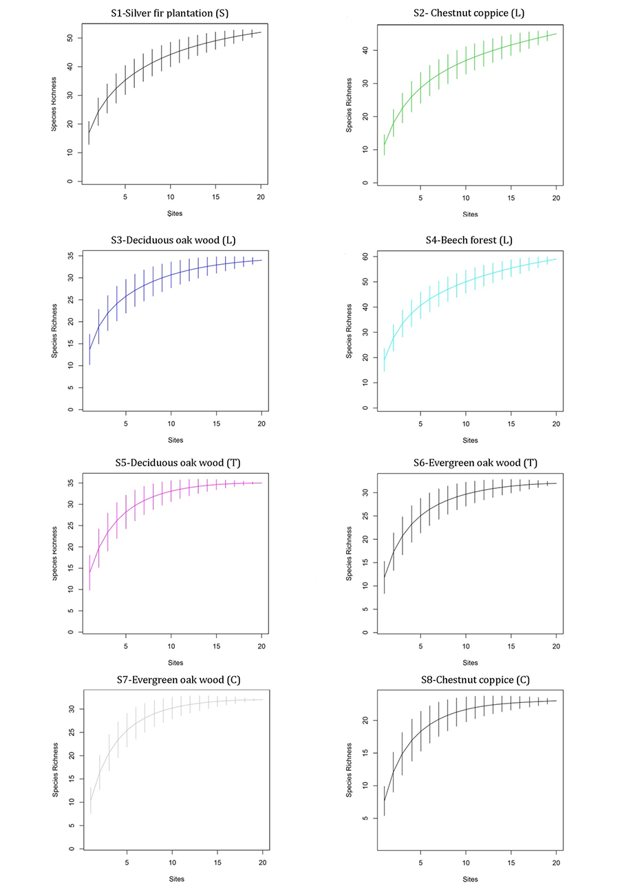
Figure 2 shows the rarefaction curves for all eight sites surveyed. Despite differing total SR, all the curves clearly show that a considerable number of species were collected. The flattened final part (the asymptote) of the curve indicates that not many species were missed.
Figure 2
The rarefaction curves for all the study sites (S1–S8). “Sites” in the graphs refer to surveyed plots in each site. (S) – Sardinia; (L) – Liguria; (T) – Tuscany; (C) – Campania.
The Species Conservation Value Index (SCVI) value ranged from the minimum in Site 6 (SCVI = 2.06 ± 0.55) to the maximum value at Site 1 (SCVI = 3.13 ± 1.1). All sites showed very similar values, except for S1 (the highest value) (Table 2).
The computed Biomass Index values (BI) ranged from the lowest (BI = 2,122.64) for Site 4 to the highest value obtained for Site 1 (BI = 45,240.036) (Table 2).
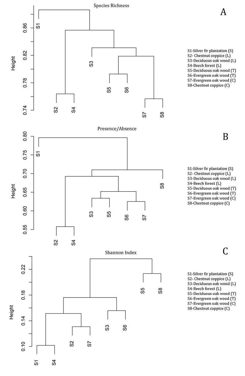
Cluster analysis (Figure 3) was plotted on SR, presence/absence data, and Shannon Index among all 160 plots. The results clearly show that sites (1–8) formed distinctive clusters, especially based on SR and presence/absence values. Moreover, Site 2 and Site 4 form a single cluster based on both SR and presence/absence data (Figure 3A,B). In contrast, the dendrogram based on Shannon Index showed different clusters among the sites (Figure 3C).
Figure 3
Cluster dendrograms of the eight sites based on macrofungal species richness (A), presence/absence (B) of species, and Shannon Index (C). (S) – Sardinia; (L) – Liguria; (T) – Tuscany; (C) – Campania.
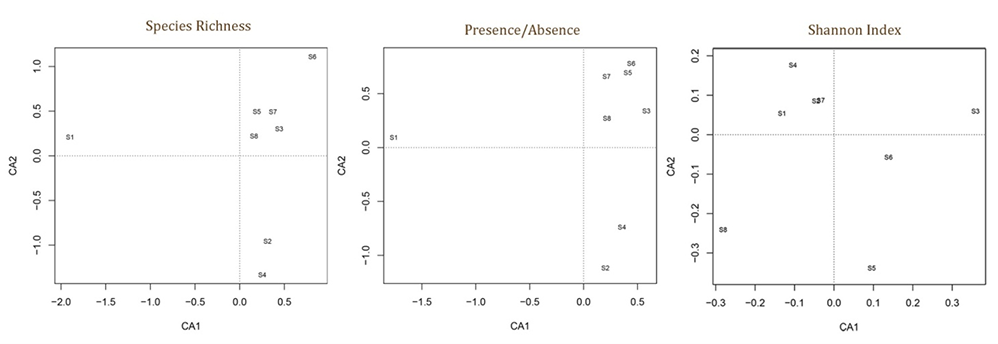
The results of the correspondence analysis are shown in Figure 4, where sites (1–8) were distributed in the multivariate space on the basis of their macrofungal SR, presence/absence of species, and Shannon Index.
Figure 4
Graphical representation of correspondence analysis of the eight sites based on macrofungal species richness (on the left), presence/absence (middle) of species, and Shannon Index (right).
The ISA results (Table 3) emphasize that some macrofungal species have a significant indicator value (IV). Specifically, we found that 13 common species were statistically significant: Armillaria mellea, Boletus aereus, Entoloma rhodopolium, Gymnopus fusipes, Hebeloma crustuliniforme, Hydnum rufescens, Inocybe geophylla, Lactarius zonarius, Marasmius oreades, Mycena crocata, Tricholoma bresadolanum, T. saponaceum, and T. ustale (Table 3).
Table 3
Summary of indicator species analysis.
| Species | Site | Vegetation | Forest type | IV | p |
|---|---|---|---|---|---|
| Armillaria mellea | S3 | Deciduous oak wood | Natural | 1 | 0.03* |
| Boletus aereus | S7 | Evergreen oak wood | Natural | 0.655 | 0.030* |
| Entoloma rhodopolium | S6 | Evergreen oak wood | Natural | 0.783 | 0.020* |
| Gymnopus fusipes | S2 | Chestnut coppice | Managed | 1.000 | 0.05* |
| Hebeloma crustuliniforme | S4 | Beech forest | Natural | 0.973 | 0.01** |
| Hydnum rufescens | S8 | Chestnut coppice | Managed | 0.894 | 0.005** |
| Inocybe geophylla | S2 | Chestnut coppice | Managed | 0.975 | 0.05* |
| Lactarius zonarius | S7 | Evergreen oak wood | Natural | 0.655 | 0.030* |
| Marasmius oreades | S7 | Evergreen oak wood | Natural | 0.845 | 0.005** |
| Mycena crocata | S4 | Beech forest | Natural | 0.964 | 0.03* |
| Tricholoma bresadolanum | S1 | Silver fir | Planted | 0.933 | 0.05* |
| Tricholoma saponaceum | S6 | Evergreen oak wood | Natural | 0.966 | 0.005** |
| Tricholoma ustale | S8 | Chestnut coppice | Managed | 0.775 | 0.035* |
Table 4 shows the biodiversity indices computed in Sites 2, 3, and 4 surveyed over 3 consecutive years (2012, 2013, 2014). Appendix S9–Appendix S14 list the recorded macrofungal species and the sporocarp abundance in Sites 2–4 (2012–2014). For all three sites, we observed the lowest index values during the third survey year (2014) (Table 4). Appendix S15 summarizes the full climate data of Sites 2, 3, and 4. Mean monthly temperatures ranged from −2.08 °C (February 2012) to 21.74 °C (August 2012), from 0.48 °C (February 2013) to 21.57 °C (August 2013), and from 3.26 °C (January 2014) to 20.06 °C (August 2014). Mean rainfall ranged from 1.8 mm (June 2012) to 348.8 mm (November 2012), from 29.8 mm (June 2013) to 416.8 mm (December 2014), and from 50 mm (September 2014) to 676 (November 2014).
Table 4
Summary of biodiversity indices in S2, S3 and S4 over three consecutive years (2012–2014).
[i] SR – species richness; pA – population abundance; pd – population density; H′– Shannon Index; E – Pielou Evenness Index; D – Simpson’s Index; d – Berger–Parker Index; Chao – nonparametric estimator Chao1; Jack. 1 – jackknife first order – nonparametric estimator; Bood. – bootstrap – nonparametric estimator; SCVI – Species Conservation Value Index; SD – Standard deviation; BI – Biomass Index; L – Liguria.
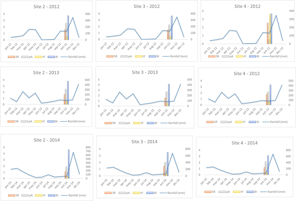
The results of PCA are shown in Table 5. Mean temperature and rainfall had a statistically significant influence on macrofungal biodiversity indices (SR, pA, H′, and BI) observed at the three sites (2–4) over 3 consecutive years. Finally, in Figure 5 and Figure 6, climatic data were compared with the selected biodiversity indices, expressed on a logarithmic scale, since they are expressed in different measurements.
Table 5
Results of principal correspondence analysis.
| PC1 | PC2 | r2 | p (>r) | |
|---|---|---|---|---|
| Temperature (°C) | 0.81090 | 0.58518 | 1 | 0.000999*** |
| Rainfall (mm) | −0.81090 | 0.58518 | 1 | 0.000999*** |
Figure 5
Graphical comparison of mean monthly temperatures detected during each surveyed year (2012–2014) in Sites 2, 3, and 4 with macrofungal biodiversity indices (in logarithmic scale). SR – species richness; pA – population abundance; H′ – Shannon Index; BI – Biomass Index. Temperatures are expressed in °C.
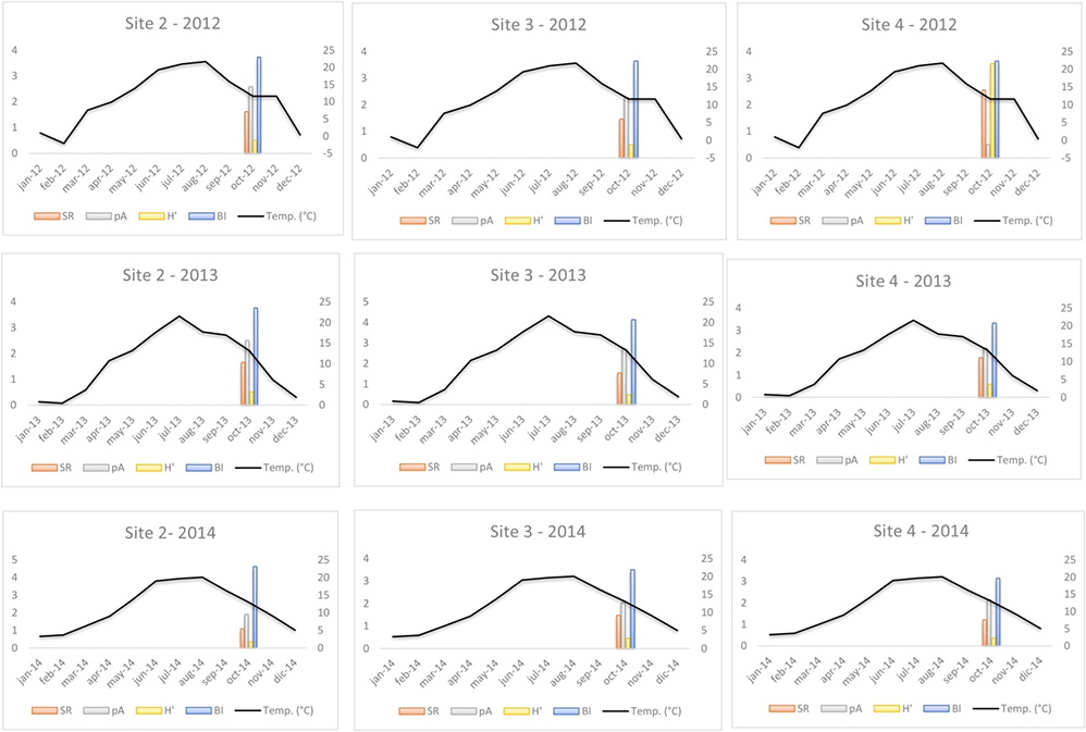
Figure 6
Graphical comparison of mean monthly rainfall detected during each surveyed year (2012–2014) in Sites 2, 3, and 4 with macrofungal biodiversity indices (on a logarithmic scale). SR – species richness; pA – population abundance; H′– Shannon Index; BI – Biomass Index. Rainfall is expressed in mm.
. Discussion
The results obtained in this study support our first hypothesis, that is, in the same surveyed time – 2013, different Mediterranean forests can differ in biodiversity quality index values (Table 1). Specifically, by comparing species richness results and their estimators (here, Chao, jackknife, and bootstrap), we can observe that the silver fir plantation (S1) and the beech forest (S4) show higher SR values than the evergreen and broadleaf oak woods (e.g., S3, S5–S7) or chestnut coppices (S2, S8). However, the estimator results confirmed that despite a large number of species being collected at each site (see rarefaction curves; Figure 2), the number of expected species in the sites is consistently underestimated (e.g., for S1). These results confirm that knowing how many species occur in a community, an ecosystem, or in a geographic area, is still a major task in ecology, even if the sampling approach is suitable (Feest, 2006) and sampling effort is exhaustive (Ambrosio et al., 2018). SR is traditionally used as a direct indicator of the level of biodiversity, but there is no consensus on how it should be estimated (Chiarucci, 2012; Xu et al., 2012). To overcome this, ecologists have devised many quantitative indices (e.g., Shannon, Evenness, Simpson’s, and Berger–Parker indices) that combine the effect of the total SR, occurrence, and evenness. Our results confirm that the silver fir plantation (S1) and beech forest (S4) showed the highest values of diversity (H′ and D), followed by the evergreen and broadleaf oak woods (e.g., S3, S5–S7) and chestnut coppices (S2, S8).
Data obtained on population abundance (pA in Table 1) and density (pd) (here, individuals are fruiting bodies/sporocarps per species) show a different scenario: Sites with lower SR and/or H′ (e.g., S3) show higher pA or pd values. Conversely, sites with high SR and/or H′ (e.g., S4) show low pA or pd values, so that sites are species-rich but sporocarps-poor. In addition, Biomass Index (BI) values do not completely reflect the SR results of sites (only S1 shows the highest SR and BI values). These results suggest that the ecology and habitat of macrofungi should also be considered. Many macrofungi can have a large size, others medium or small size, and they can grow in a dense cluster, gregarious or as “solitaries.” Hence, the BI value of a site can provide an indirect indicator of the occurrence of macrofungal communities within the given site. Moreover, for the purposes of prioritizing the conservation of sites, based on their level of diversity, compound indices are often preferred over SR, as the complexity of biodiversity cannot be encapsulated by a single number (Ambrosio et al., 2018; Feest, 2006; Gaston & Spicer, 2004).
Site community similarity was tested by both H-CA and CA considering the value of SR, presence/absence of species, and Shannon Index in each surveyed plot and site (Figure 3 and Figure 4). The results show that patterns of site distribution are driven by a geographical gradient (e.g., geographic distance) and vegetation type (Figure 3). The dendrograms in Figure 3 indicate that sites form distinctive groups on the basis of the vegetation and geographic distance. All these results support our first hypothesis that different Mediterranean forest types show different macrofungal biodiversity quality values. Both the silver fir plantation (S1) and beech forest (S4) showed different values and patterns of distribution from those of the other sites. Conversely, within the same vegetation type, sites show more statistical similarities: the evergreen and broadleaf oak woods (S3, S5–S7) or chestnut coppices (S2, S8) form very close (clustered) groupings. By considering forest management, we observed that unmanaged sites had higher macrofungal biodiversity values than the managed sites (S2, S8). These results agree with those of other studies (see Tomao et al., 2020) that recognize that unmanaged forests (especially when they evolve to old-growth forests) are reserves of high fungal SR and diversity. Tomao et al. (2020) also affirmed that some silvicultural practices can negatively affect fungal diversity and dynamics (in our case, S2 and S8).
To assess the effect of climate conditions (temperature and rainfall) (our second hypothesis), we compared these factors with various biodiversity indices (SR, pA, H′, and BI) recorded at three sites (2–4) over 3 consecutive years (2012–2014) (Figure 5, Figure 6, and Table 5). Both climatic variables were statistically significant in relation to the biodiversity indices (Table 5). However, we observed that during the third year of surveys (2014), we measured the lowest index values. Overlapping these results with monthly temperatures and rainfall data, we can observe that 2014 was hotter than 2013 and 2012, and the mean rainfall was lower than in the previous years, especially in summer and early fall. These results confirm that at the same site, surveyed over consecutive time periods, climatic variations can affect the composition of macrofungal communities. Several studies (Büntgen et al., 2011, 2013; Egli, 2011) confirmed that seasonal macrofungal yield is influenced positively by precipitation amounts and mean temperatures, especially by spring–summer temperatures and total precipitation from September to October. Inter-annual fluctuations and long-term trends in the formation of fungal fruiting bodies, as well as intra-annual shifts in the timing of their productivity, have been related to land/use-cover change (including deforestation), increased harvesting, and pollution (Büntgen et al., 2011, 2013; Tomao et al., 2020). Hence, macrofungi and measurements of their biodiversity can be useful indirect indicators of inter- and intra-annual climate changes.
The specific habitat requirements of fungi and influence of biotic and abiotic factors on their growth make them well suited as indicators for selecting conservation areas and monitoring their status. Notoriously, northern European studies (Heilmann-Clausen et al., 2014) emphasized the role of wood-inhabiting fungi (e.g., polypores) as useful indicators of forest perturbations (e.g., the lack of old trees and dead wood); however, on the basis of our results and other studies performed in South Mediterranean forests (i.e., Ambrosio & Zotti, 2015), we suggest that epigeous Agaric, Bolete, and Gasteromycete macrofungi should be considered as useful habitat indicators (Table 3) because they are highly sensitive in detecting changes in ecosystems (e.g., N deposition; Feest et al., 2014). Moreover, the calculation of a statistical index (SCVI; Table 2 and Table 4) can provide indirect information about the presence of rare species. In our study, Site 1 showed a higher SCVI value, indicating the presence of rare species, compared to other sites, and its value remained stable (see Table 4) over time, despite poor rainfall. Several indicator schemes based on fungi have been suggested for assessing the conservation value of forests and grasslands (Feest, 2013); however, biodiversity conservation initiatives till date have often overlooked the pivotal role of fungi in biodiversity monitoring (Heilmann-Clausen & Vesterholt, 2008).
In conclusion, the results of this study represent the ecological contribution and role of the quality of macrofungal biodiversity as a predictor of Mediterranean forest health and dynamics. The results obtained show that Mediterranean forests, while briefly investigated, show different macrofungal biodiversity indices influenced by forest type and management. Inter- and intra-annual temperatures and rainfall fluctuations affected the formation of fungal fruiting bodies (sporocarps) and consequently the dynamics of communities. Based on these results and published literature, it is possible to confirm the ecological response to climate variations reported for a broad range of taxa, including macrofungi. Preserving fungal diversity in forest ecosystems is important because of the positive relationship between fungi and ecosystem multifunctionality, as well as their potential early role as indicator species. Mycorrhizal fungi, in particular, synergistically affect plant communities and ecosystem services through altered functional traits and ecology of host plants (Tedersoo et al., 2020).
Preserving and restoring forests and improving predictions about the impacts of global change and pollution on vegetation and soil processes, by both direct and indirect indicators, means guaranteeing the conservation of the most bio-complex ecosystems and related ecological processes that are the basis of future life on Earth.
. Supplementary Material
The following supplementary material is available for this article:
Appendix S1: List of recorded species in Site 1 (in 2013).
Appendix S2: List of recorded species in Site 2 (in 2013).
Appendix S3: List of recorded species in Site 3 (in 2013).
Appendix S4: List of recorded species in Site 4 (in 2013).
Appendix S5: List of recorded species in Site 5 (in 2013).
Appendix S6: List of recorded species in Site 6 (in 2013).
Appendix S7: List of recorded species in Site 7 (in 2013).
Appendix S8: List of recorded species in Site 8 (in 2013).
Appendix S9: List of recorded species in Site 2 (in 2012).
Appendix S10: List of recorded species in Site 2 (in 2014).
Appendix S11: List of recorded species in Site 3 (in 2012).
Appendix S12: List of recorded species in Site 3 (in 2014).
Appendix S13: List of recorded species in Site 4 (in 2012).
Appendix S14: List of recorded species in Site 4 (in 2014).
Appendix S15: Mean monthly temperatures and rainfall recorded in Site 2, 3, and 4 in 2012, 2013, and 2014.