Germplasm and Phenotyping

For the purposes of this study, we assessed 32 Tunisian barley lines (Hordeum vulgare L.) comprising four cultivars developed by the Tunisian breeding program in collaboration with ICARDA (Rihane, Manel, Lemsi, and Kounouz), one accession with uncertain improvement status, and 27 landraces. All accessions were obtained from the U.S. National Plant Germplasm System international database. According to passport data, the 28 accessions other than the aforementioned four cultivars were collected or donated from Tunisia between 1922 and 1972 (Table 1). During the three cropping seasons of 2016/2017, 2017/2018, and 2018/2019, field trials were conducted in El Kef, Tunisia, which is characterized by a semiarid climate with an average annual rainfall of 380 mm (Table 2). Each accession was planted in two replicate plots, each comprising two 2.5-m-long rows planted with 65 seeds with an inter-row spacing of 25 cm. With the exception of yield, all assessed traits were measured from five plants. The traits evaluated in this study were as follows: grain yield: the weight of grain harvested from the two rows; plant height: measured from the soil surface to tip of the spike (excluding awns); days to heading: the number of days from sowing to the time when 50% of the ear had emerged; peduncle length: measured from the base of the spike to the flag leaf node; internode length: measured from the flag leaf node to the next node; awn length: the length of the awn in the central spikelet; spike length: measured from the base of spike to the tip of the terminal spikelet (excluding awns); and kernel number per spike: the number of grains per spike.

Statistical Analysis of Phenotypic Data

For each trait, descriptive statistical data were obtained based on the average barley accession data. We used the following additive main effects and multiplicative interaction model that combines two standard methods, namely, analysis of variance (ANOVA) with principal component analysis (PCA) analysis (Zobel et al., 1988):

where Y_ijr is the phenotypic trait, µ is the grand mean, g_i is the main effect of the ith genotype (G), and e_j is the main effect of the jth environment (E). λ_k is the singular value for the interaction principal component (IPC) axis, k, α_ik and γ_jk are the genotype and environment IPC scores (i.e., the left and right singular vectors) for axis; k, b_r(e_j) is the effect of block r within environment j, r is the number of blocks (in this study, the number of blocks was not considered, and thus, the effect of blocks was removed), ρ_ij is the residual containing all multiplicative terms not included in the model, n is the number of axes or principal components retained by the model, and ε_ijr is the experimental error, assumed to be independent of the distribution ε_ij ∼ N (0, σ).

Analysis of the additive main effects and multiplicative interaction model and the genotype main effects and Genotype × Environment interaction effects model were performed using Genotype × Environment Analysis with R software in Windows (Pacheco et al., 2016).

Descriptive Statistics

Basic statistical parameters for each of the three growing seasons (mean, standard deviation, minimum, and maximum values) for the barley accessions are summarized in Table 4. Almost all traits showed an increase in mean values over the three cropping seasons; for example, mean grain yield increased from 368.5 g in 2017 to 457.8 g in 2019, and plant height increased from 68 cm to 102.5 cm. In contrast, there was a delay in the heading date from 123 days in 2017 to 131 days in 2019.

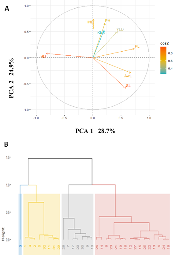
PCA analysis revealed that 68.7% of the phenotypic variation could be explained by the first three components, with the first two components, PCA1 and PCA2, explaining 28.7% and 24.9% of the total variation, respectively (Figure 1A). Heading date and spike length were found to be major contributors to these two components, whereas among the assessed accessions, kernel number per spike exhibited the lowest contribution to the total phenotypic variation. Hierarchical clustering based on the mean value of the target traits over the three cropping seasons grouped the accessions into four clusters (Figure 1B). The Lemsi cultivar was considered to represent a discrete group, on account of its late heading and awnless spike. The other modern varieties were grouped in the second cluster, the constituents of which were characterized by tall plants with higher yields. The third cluster group comprised medium-tall plants with low yield and late heading, whereas the fourth group contained early heading short-statured accessions.

Figure 1

Principal component (A) and hierarchical cluster (B) analyses. The first two principal components, PCA1 and PCA2, explained 28.7% and 24.9% of the total variation. Days to heading (DH) and spike length (SL) make the major contributions to the total variation. Hierarchical cluster based on the mean values of the studied traits across the three cropping seasons identified clusters of accessions. See the text for explanation of other abbreviations.

The phenotypic correlations of the studied traits across the three cropping seasons are presented in Table 4. The combined data obtained over the three seasons revealed that heading date was negatively correlated with almost all other traits, with the exception of plant height. Plant height was found to be significantly positively correlated with grain yield (r = 0.45, p < 0.05), but it was negatively correlated with spike length.

Analysis of Variance

The results of analyses of variance for the grain yield-related traits of each genotype in each growth season based on interaction effects are presented in Table 5. Total variance among the genotypes, environment (seasons), and interaction effects was found to be highly significant (p ≤ 0.01). For heading date, spike length, kernel number per spike, awn length, and yield, genotypic effects were found to be considerably stronger than the environmental effects, ranging from 35.6% to 66.9%. The effect of the interaction between genotype and environment on yield was important for yield (48%), although similar effects were relatively small with respect to heading date (9.9%) and plant height (8.14%). A large phenotypic variation explained by genotypes indicated the diversity of the genotypes and that a major fraction of the observed variation in heading date and spike length could be attributed to genetic effects.

Analysis of Stability and Genotype by Environment Interaction Effects

Stability parameters are useful for characterizing genotypes by indicating their relative performance in different environments. In the present study, we combined the data for yield and yield-related traits for all three cropping seasons with stability statistics by measuring the Shukla variance (Shukla et al., 1972) (Table 6).

It was accordingly found that accession G20 with the smallest coefficient of variability (−207) was the most stable genotype in the selection ranks for yield across the three cropping seasons; however, there were a further 11 genotypes selected based on higher yield and small coefficient of variance (Rihane, Manel, G12, G13, G14, G16, G23, G25, G29, G31, and G32).

The number of genotypes selected based on coefficient of variability (s²_di) ranking varied among the traits. Two accessions (G13 and G17) were found to be stable with respect to heading date; two (G18 and G20) were stable for plant height; four were stable for spike length (G7, G24, G25, and G30); and two were stable in terms of awn length (G3 and G27).

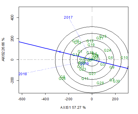
The classification of genotype instability attributable to environmental variability highlighted the need for further detailed studies on the behavior of these accessions during selection of the best genotypes. To visualize the performance of different genotypes in a given environment, we constructed biplots. The first two main factors (components) of the biplot analysis was applied to the Genotype × Environment interaction and explained 83.9% of the total variation, thereby indicating that biplot graphics explain most of the sums of squares and Genotype × Environment interactions with respect to genotype. The lines (blue lines) that connect the test environments to the biplot origin are referred to as environment vectors. The cosine of the angle between the vectors of the two environments approximates to the correlation between these environments. Environment 2017 (E2017) and E2018 were found to be positively correlated (acute angle) and E2018 and E2019 were highly correlated, whereas E2017 and E2019 appeared to be uncorrelated (right angle) (Figure 2). The close associations detected among test environments indicate that we can obtain similar information regarding genotypes. The concentric circles on the biplot enable visualization of the length of the environmental vectors, which provides a measure of environmental discrimination. Accordingly, the two years 2017 and 2018 show similar vector lengths and are thus considered discriminating and informative environments, whereas 2019 was found to be less informative. The smaller the angle of the environmental vector with the AED (average-environment axis) (Figure 2), the more representative it is of other test environments. Thus, E2017 and E2018 were found to be the most representative, whereas E2019 was the least representative. Environments such as E2017 and E2018 that are both discriminating and informative are considered good environments for selecting generally adapted genotypes. The pattern of the environments in the aforementioned biplots is indicative of two mega-environments, one of which one is a semiarid climate represented by E2017 and E2018, and the other is a subhumid climate represented by E2019.

Figure 2

Discriminativeness vs. representativeness of the three evaluated cropping seasons. The first two main factors (components) of the biplot analysis applied to Genotype × Environment interaction effects explained 83.9% of the total variation. Environments 2017 and 2018 were positively correlated (acute angle) and 2018 and 2019 were highly correlated, whereas 2017 and 2019 were uncorrelated (right angle).

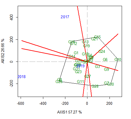
A set of perpendicular lines divided the which-won-where biplot into multiple groups (Figure 3). A polygon was initially drawn to encompass all genotypes. Thereafter, lines perpendicular to each side of the polygon were drawn, starting from the biplot origin. The perpendicular lines radiating from the origin of the biplot divide the plot area as well as the test location into sectors. Note the red lines and genotypes in the vertex of the polygon, and the lines dividing the sectors, indicating the mega-environments. The best genotype in each mega-environment corresponds to the vertex; for example, in the sector representing E2018 and E2019, the genotypes G8 and G26 have the best yield, whereas in the sector representing E2017, G12 and G16 have the best yields.

Figure 3

A which-won-where biplot. In the sector within which environments 2018 and 2019 are plotted, the genotypes G8 and G26 have the highest yields, whereas in the sector in which environment 2017 is plotted, G12 and G16 have the highest yields.

We subsequently evaluated the 32 assessed genotypes for mean performance and stability across environments (Figure 4). The single-arrowed line is the average-environment coordination abscissa, which indicates a higher mean yield across environments. Accordingly, the plot shows that accessions G8 and G26 had the highest mean yield, followed by G12 and G16, whereas G10 and G30 had the lowest mean yields.

Figure 4

A Genotype × Environment interaction effects biplot representing the Means × Stabilities that indicate the yield rankings of the 32 assessed barley accessions. Accessions G8 and G26 have the highest mean yields, followed by G12 and G16, whereas G10 and G30 have the lowest mean yield. Genotype G8 and G26 were highly unstable, whereas G20 and G22 were highly stable.

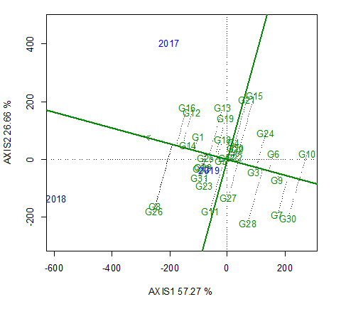
The higher the genotype projection on the axis, the lower is the genotype by environment interaction, and consequently, the more stable the genotype. Thus, genotypes G8 and G26 were identified as being highly unstable, whereas G20 and G22 are considered highly stable.