Introduction
Diagrammatic or graphical illustration of contemporary knowledge of life in a single figure has long been sought in biological sciences, particularly in botany. The first part of this article presents a short historical account of illustrations devoted entirely to plants. The main types of diagrams are summarized by referring to their first uses in plant sciences and the advantages and disadvantages of each graphical approach are outlined. A major shortcoming of diagrams published thus far is that they focus on only a single or a few relevant aspects of the plant world at a time. While classification is always present, morphological or phylogenetic affinities, fossil taxa, the geological timescale, and the diversity of taxonomic groups are never shown simultaneously and reliably. This problem can be resolved using an old/new type of images – the coral. It is old in the sense that C. R. Darwin was the first to state that the coral is perhaps a better simile of evolution than trees but new in the sense that its mathematical properties and possibilities of its application in contemporary science have only been introduced and revealed recently. The theoretical background of and certain practical problems associated with the compilation of the Coral of Plants are discussed in the second part. The Coral of Plant Life is displayed as two separate figures for didactic and technical reasons: the evolutionary timescale is much longer, and the extant diversity is much lower for red and green algae than for embryophytes.
Visualizing the Plant World – A Brief Historical Account
Several authors, notably Ragan (2009), Tassy (2011), Kutschera (2011), Pietsch (2012), and Archibald (2014), have reviewed how the tools of visualizing organismal life evolved over time, mostly with reference to the Tree of Life. Although the iconography of the entire living world on Earth is in focus, these articles and books are somewhat biased toward zoological systematics and anthropology and exclusively botanical diagrams receive less attention. For example, only five of the hundred or so figures by Archibald (2014) or only 38 of the 230 figures by Pietsch (2012) illustrate plant systems. Moreover, I believe that the iconography in these studies is incomplete and incoherent; thus, a short summary of the history of visualizing only botanical knowledge is in order. As will be demonstrated, the diagrammatic representations of plant life are limited in scope and depth and take various forms. They range from text-dominated tabular arrangements with very few graphical elements, through botanical metaphors (trees, shrubs, or cacti), to proper mathematical constructs, such as graph theoretical trees and networks.
Of note, this chapter is not meant to be a complete review, which would be beyond the scope of the present article. Nevertheless, to the best of the author’s ability, the most interesting and relevant pictures from the history of botany were selected. All figures discussed in this section are collated in Appendix S1, together with references to the studies in which they appeared.
Scala Naturae – An Exclusive Hierarchy
For almost two thousand years, the Platonian/Aristotelian view, which suggested that natural objects can be arranged into the Great Chain of Being (scala naturae), prevailed in science. This is an exclusive hierarchy in which one group is positioned under the other, implying lower- and higher-order relationships, often illustrated using a ladder-like diagram. In its original form proposed by Aristotle, the single group of plants included all living beings that cannot move and exhibit senses but can grow and reproduce. Even in the most elaborate versions of the Great Chain of Being, plants are under-represented compared with inanimate objects and animals. For example, in 1745, C. Bonnet used only six groups for organisms that were considered plants at the time, from truffles to sensitive plants, and dedicated 25 steps of the ladder to animals and over 10 steps to inorganic materials (Figure S1).
Bracketed Tables – Inclusive Hierarchies
The Aristotelian logic also influenced the way natural objects were arranged in a single diagram, resulting in a system quite different from the scala. In this alternative system, the supreme genera (categories corresponding to large groups) are subdivided into subordinate genera (smaller groups) using a given differentia specifica and the latter genera are further subdivided according to other criteria, and so on, right down to individuals. This divisive process produces an inclusive hierarchy – a nested system of objects in which smaller groups are embedded within larger ones. Aristotle’s method of logical division was first demonstrated visually via the Porphyrian tree (Figure S2). When applied to organisms, the idea of lower and higher groups was abandoned; animals and plants are now positioned at the same level and, similarly, animals and humans are positioned at another level, as seen in the most-often cited example of the method (Figure S3). Such hierarchies appear in early botanical classifications of several smaller taxa, such as grasses, prepared by P. Pena and M. de l’Obel [Lobel] in 1571 (Figure S4), and orchids, prepared by M. de l’Obel in 1576 (see Pietsch,2012). These early authors used the so-called bracketed tables in which an initial group is successively subdivided into smaller ones, such that the labels and descriptions of each subdivision are connected by curly brackets. Almost simultaneously, and quite naturally, in 1592, A. Zaluziansky adopted the method of logical division in plant identification keys for several taxa in Methodi Herbariae Libri Tres (Griffing,2011) (Figure S5). Subsequently, tabular arrangements with brackets were used as both identification keys and classification systems, extended to the entire plant world known at the time. A classic example of this is the “Clavis systematis sexualis” of plants from the first edition of Systema Naturae by C. Linnaeus in 1735 (Figure S6). The figurative element of brackets, together with tabular listings, remained popular for a long time, as exemplified by the dichotomous key to the French flora drawn by J.-B. Lamarck in 1778 (Figure S7) and the class-level plant classification suggested by A. L. de Jussieu in 1789 (Figure S8).
Networks and Maps
Hierarchical classification can be converted to a graph theoretical tree: exclusive hierarchies into linear trees and inclusive hierarchies into dendrograms. However, several botanists were not satisfied with such arrangements, claiming that affinities among different groups can only be illustrated sufficiently using network-like structures. Noted examples include the diagram of plant orders drawn by J. Ph. Rühling in 1774 (Figure S9) and the “affinity table” proposed by A. J. G. C. Batsch in 1802 (Figure S10). While the first one is predominantly tree-like, with connections added between terminal groups, the latter one is overwhelmed by interconnections and, therefore, very confusing and difficult to interpret. As another solution to depicting affinity relationships, P. D. Giseke prepared a map-like figure for Linnaeus’ book published posthumous in 1792 in which each taxon was represented by a circle and groups with close affinity were positioned near one another (Figure S11). To the best of my knowledge, it is the first graphical visualization of the diversity of taxonomic groups: The diameter of each circle is approximately proportional to the number of genera in the respective taxon.
Nonevolutionary Figurative Trees
Figurative or proper trees are those resembling the silhouette of the real one. Botanical trees have long been popular in different areas of humanities to illustrate, for example, the genealogy of royals, giving rise to the common term “family tree.” Such diagrams have also been frequently used for summarizing knowledge in various fields of science, such as in the French Encyclopedia (Hellström,2019). In the history of botany, A. Augier was the first to attempt summarizing his own hierarchical plant classification using a figurative tree (“arbre botanique”; Figure S12) in 1801. In this, the leaves were the smallest units of classification he has shown, corresponding to families, which were successively joined to twigs and branches (classes and tribes, respectively). In demonstrating details of the categorization of plant world into classes, and the subdivisions within each of the 20 classes, Augier used the well-known bracketed table style throughout the book. The hierarchy was not fully inclusive, however, because some of the larger groups (tribes, classes, and even orders) were positioned one under the other on the main trunk and branches, reminiscent of the manner in which groups are arranged in the scala naturae.
Although there are suggestions (e.g., Lecointre,2015) that Augier’s tree might have a temporal aspect, figurative trees receive explicit time dimension first in E. Hitchcock’s book published in 1840 (Figure S13). His tree-like figure – the “paleontological chart” – summarizes the appearance and relative species richness of major plant (and animal) groups in different geological ages. Although the diagram shows several bifurcations potentially indicating evolutionary divergence, mostly for animals, Hitchcock was in favor of gap creationism, dismissed the theory of evolution, and thought it better to remove the figure from latter editions of his book to avoid any phylogenetic connotation. In fact, as Hitchcock himself admitted (Archibald,2009), the first figure ever to incorporate three basic types of information, namely classification, diversity, and geological time, appeared 3 years earlier. In 1837, H. G. Bronn placed spindle-like shapes into the time dimension to illustrate changes in species richness of taxa over time and included some plant groups in these diagrams (Figure S14A,B). A similar figure devoted entirely to major plant groups was drawn by the paleobotanist L. F. Ward in 1885, which was subsequently modified in A. R. Wallace’s book on Darwinism published in 1889 (Figure S15A,B). In these diagrams, all shapes run parallel to one another without links, showing that the authors had not yet attempted to depict phylogenetic relationships, even though both were strong supporters of the theory of evolution.
Graphs, Trees, and the Notion of Change
Genealogy in the plant world was first illustrated by A.-N. Duchesne as early as 1766, through a network for a very small group of strawberry varieties (Pietsch,2012, his Figure 20). However, the notion of change had escaped the attention of botanists for a long time, and evolutionary and phylogenetic thinking was primarily restricted to zoology. Relevant illustrations referred only to animals in the works of Lamarck, in the notebooks of Darwin (who never published trees for living organisms), and in publications of other pioneers of the theory of evolution, such as C.-H. de Barbancois and R. Chambers. Plants become emphasized in some of the several phylogenetic diagrams designed by the notorious tree-maker E. Haeckel. One of the three main limbs in his famous “Monophyletischer Stammbaum” from 1866 corresponds to plants. In this, extant groups appear as terminal twigs of an oak-like figurative tree (Figure S16). He also produced various other forms of figurative or metaphorical trees for plants in which extant groups remained as terminal twigs and geological time was indicated as well (Figure S17A). In yet another attempt in the same book as the Stammbaum, Haeckel displayed plant phylogeny in which both extinct and extant groups were terminal twigs (Figure S17B). As a further proof of his struggles with phylogenetic imagery, Haeckel also drew a bona fide graph theoretical tree of plant life in which the main axis corresponded to a sequence of large groups, like in the scala naturae (grade tree; Figure S18). In plant phylogenetics, this was the first illustration of evolutionary gradualism with added ramifications. This dual idea continued to exist much later into the twientieth century: The phenomenon that higher Linnaean taxa are derived from each other combined with bi- or multifurcations occurred most frequently in diagrams showing angiosperm phylogeny, starting with H. Hallier’s “arbre genealogique” in 1912 (Figure S19) and C. E. Bessey’s “cactus” diagrams in 1887 and 1915 (Figure S20A,B) and ending with A. L. Takhtadjan’s and A. Cronquist’s figures in the 1980s (Figure S21A,B).
Spindle Diagrams
Another figure drawn earlier by Bessey in 1887 (Figure S22) had peculiar features: The diversity of each dicot taxon was visualized as triangles of different size (similar to the shapes in his cactus) and the change in richness of each taxon over three geological time periods was illustrated as a nested arrangement of these triangles. This idea to depict phylogeny, classification, time, and diversity simultaneously was novel, although the complexity of his diagram made it less efficient for visualization. A simpler solution was achieved by modifying and expanding the figures of Bronn and Hitchcock according to the theory of evolution, resulting in the so-called spindle diagrams.12 In these diagrams, geological ages are shown on the vertical axis and the taxa are spindles or bubbles of various shapes and length, roughly illustrating changes in diversity over time. However, the width of spindles is rarely, if ever, proportional to the number of species (or other taxa) in the given group, and different spindles are hardly comparable even within the same figure. The spindles are connected to illustrate phylogenetic relationships, although these links are uncertain (dotted lines) or even missing in many cases. If present, the links imply ancestor–descendant relationships between higher (Linnaean) taxa – a feature characteristic of gradistic phylogenetic thinking. Noted examples of spindle diagrams in botanical classification include those prepared by W. Zimmermann in 1930 for various groups of plants as well as for the entire plant world (Figure S23). Along the same lines, in 1955, H. J. Lam prepared a similar figure for cormophytes, including many details concerning fossil taxa (Figure S24). Spindle diagrams remained popular for a relatively long time in taxonomic and paleobotanical works, for example, in Stewart and Rothwell (1993, their Charts 11.1, 16.1, 20.1, 26.1, and 30.1), DiMichele and Bateman (1996, their Figure 1), and Sokoloff et al. (2015, their Figure 2).
Cladograms
As mentioned above, the notion that contemporary taxa are endpoints and the branching pattern of the tree refers to their evolutionary past, appeared in Haeckel’s oak-like tree (Figure S16) which be considered the earliest, albeit unintentional and weak, sign of cladistic thinking in the history of biology (Archibald,2014; Podani,2017). In botany, a further significant step in this direction is the evolutionary tree prepared for the Compositae family by J. Small in 1919 (Figure S25). In this tree, all tribes appear as endpoints, information on the geographic distribution of taxa appears at the internodes, and the geological timescale is added as the vertical axis. Despite its predominantly cladistic appearance, the diagram includes some anastomosing links (Morrison,2013) as indicators of hybridization; therefore, this picture cannot be considered a true and intentional forerunner of cladism. Similarly, the tree of monocotyledonous plants drawn by F. Ankermann in 1927 (as modified by U. Hamann in 1961, Figure S26), is implicitly cladistic in most parts, although three groups near the root indicate the presence of gradistic thinking of both authors. The essence of the cladistic approach, that is the attention on sister relationships among contemporary organisms, became clear a few years later in 1931, when Zimmermann published a small tree for three plant taxa to illustrate the idea (Figure S27). Subsequently, W. Hennig’s work, specifically the English translation of his seminal book (Hennig,1966), revolutionized the entire systematics by introducing the cladistic approach (called “phylogenetic systematics” by Hennig). Its intention was to objectively reconstruct the past of a given group of organisms in the form of a cladogram, a preferably bifurcating graph theoretical tree, which then serves as the basis for classification. Since Hennig was a zoologist, early uses of cladistic analysis and the dispute over its philosophical background appeared in journals such as Systematic Zoology. In botany, studies were relatively infrequent at the beginning (Funk and Wagner,1982, provide a bibliography). In 1968, T. Koponen published the first Hennigian cladistic study11 on the moss family Mniaceae in Finland. Furthermore, in 1980, L. R. Parenti conducted the first analysis of a large plant group (practically, the current Viridiplantae) (Mishler,2014). Her cladogram (Figure S28) was a comb-shaped tree, reminiscent of the linear and gradual ordering of groups in the Great Chain of Being. In addition, it is an asynchronous cladogram (sensu Podani,2013), since both extinct and extant groups appear as terminal vertices and the implied sister relationships do not necessarily hold true.10 Meanwhile, the potential applicability of molecular sequences as a basis for reconstructing genealogical relationships among different taxa was also realized, with the first report in botany published by Boulter et al. in 1970 for five species (Figure S29). Later, molecular information rapidly became of central importance in systematics, as demonstrated by thousands of cladograms applied at various ranks in the Linnaean system as well as by progressively improved and increasingly stable synthetic cladograms for angiosperms well-documented by the Angiosperm Phylogeny Group (Angiosperm Phylogeny Group I–IV, 1998,2003,2009,2016) and for lycophytes and fern allies suggested by the Pteridophyte Phylogeny Group (2016). The weakness of cladograms, and of graph theoretical trees in general, is that the number of terminal nodes (taxa) cannot be increased beyond a certain limit without risking interpretability and readability. Mandalas and spiral trees hardly solve this problem, even though they may contain thousands of endpoints (Podani,2019).
The use of molecular data enabled two significant modifications. Topological information in synchronous cladograms may be supplemented with molecular distances measured along the edges. Such trees are often called phylograms, in which terminal nodes are at different distances from the root. The use of molecular clock, on the other hand, together with known ages of fossil taxa, allows the estimation of divergence times of sister groups and preparation of the so-called time trees or chronograms. These are cladograms embedded into the time dimension, satisfying the ultrametric inequality (indicating that for any three terminal nodes, the distances between the members of two pairs are equal and cannot be smaller than the distance between the members of the third pair).
Dendrograms of Numerical Taxonomy
The ultrametric property also holds true for diagrammatic representations of Linnaean systems (for taxonomic levels of any three species) and, most remarkably, for the standard output of numerical taxonomic (phenetic) studies, the dendrograms (phenograms) which are also graph theoretical trees. This approach was pioneered by Sokal and Sneath (1963), developed in parallel to the cladistic method, to make taxonomic analysis as objective as possible. In dendrograms, morphological (dis)similarity is measured on the vertical axis, and taxa are derived by “cutting the tree” at arbitrary levels. Most analyses are restricted to relatively low Linnaean ranks, usually genera, tribes, and families (for bibliography, see B. R. Baum et al.,1984), because at higher levels it is increasingly difficult to compile a full data matrix with homologous characters. A noted exception is the study by Young and Watson on dicots (Figure S30) performed as early as 1970 when no computers were available yet to properly handle 543 genera based on a data matrix with 83 attributes.
Unusual Representations of Phylogenetic Relationships
Sporne (1974) argued that phylogenetic trees cannot be drawn without sufficient knowledge of fossils and proposed separate circular diagrams for extant monocots and dicots. In these diagrams, the orders were represented by roundish or elongated shapes arranged in a circular manner, with length reflecting the morphological advancement of a given group from a hypothetical ancestor. Related groups are closely positioned to one another (Figure S31). Thorne (1992) stated that deriving a major group from another is misleading and suggested a similar diagram – the so-called “phyletic shrub” – as a visual means of illustrating phylogenetic classification. Essentially, it is a two-dimensional map (like Giseke’s) in which each order is represented by an irregular shape (bubble) proportional in area to the diversity of the order (Figure S32). Shapes adjacent to each other reflect close relationships, whereas their distances from the hollow center represent divergence from a supposed angiosperm ancestor, as in Sporne’s figure. This scheme may be conceived as a horizontal slice of R. Dahlgren’s three-dimensional diagram, an arrangement of diverging branches (the taxa) of different diameters and cross sections, originating from a nearly common base (Figure S33). In all these diagrams, however, the cladistic component is missing or weak; therefore, these are hard or impossible to interpret phylogenetically.
Need for a Comprehensive Diagram
The historical overview of the previous section arrives at the conclusion that different approaches to visualize knowledge regarding the plant world depict only a single or a few relevant aspects of contemporary botanical knowledge. Classification, phylogeny, chronology, paleontology, species diversity, and history of major evolutionary innovations are hardly, if ever, demonstrated simultaneously and adequately in a single image. This is shown by the following summary of the uses of different diagrams:
Bracketed tables – (pre-)Linnaean classification;
Maps and shrubs – Linnaean classification; number of species or genera in highly ranked taxa and their relative phylogenetic closeness or morphological affinity;
Networks – Linnaean classification; affinity between higher taxa or evolutionary relationships of species or categories below the species level;
Figurative trees – Linnaean classification; metaphors of phylogeny as early trees of life, occasionally embedded in geological time;
Spindle diagrams (romerograms) – Linnaean classification; temporal extent and inadequately shown relative diversity of extinct and extant taxa, weak signs of phylogeny, if any;
Cactus diagrams – Linnaean classification; phylogenetic relationships (grades) and within-group diversity;
Grade trees – Linnaean classification; phylogenetic relationships (grades) between highly ranked groups;
Cladograms – sister group relationships between taxa at the same time horizon; Linnaean or cladistic classification derived a posteriori, time (chronograms) or evolutionary distance (phylograms);
Dendrograms or phenograms – (dis)similarity of taxa, Linnaean classification derived a posteriori.
Role of Classification
Classification and the associated nomenclature are central to the subject. There would be no possibility to illustrate anything without arranging natural objects into named categories. Notably, in all but the last two cases in the above list, a given image summarizes an existing classification, whereas in phenetics and cladistics, the classification is derived from the analytical results, dendrograms, and cladograms, respectively. All traditional taxonomic approaches and phenetics agree that classifications are Linnaean (rank-based), that is, extinct and extant species are grouped into genera, families, orders, classes, and phyla, plus dozens of categories in between. However, the classificatory interpretation of cladistic results is equivocal. Many authors use molecular or morphological cladistic methods to revise the existing Linnaean classification at various taxonomic ranks to retain only “monophyletic” (or rather “monocladistic,” sensu Podani,2010) groups. In APG I–IV, the Linnaean ranks and nomenclature up to the level of orders are maintained and the use of clades and phylogenetic (rank-free) nomenclature further up is suggested. However, this practice is illogical: Ranked groups should not be used simultaneously with clades. Clades are historical entities, whereas ranks work at best in the classification of contemporary organisms such that the choice among ranks remains arbitrary. Lamarck and Darwin warned us about the latter long time ago. If the purpose of a diagram is to summarize the past and present plant life together, ranks do not work at all: Groups delineated at present cannot be projected back into the past in a meaningful way (see Podani,2010,2019, and references therein) – another topic elaborated in the present article. The solution is to switch to rank-free groups and phylogenetic nomenclature, which is a painful step for many of us so firmly accustomed to the Linnaean tradition. If we accept this suggestion and set aside the system of ranks, the following question arises: what kind of a diagram demonstrates as many aspects of life as possible, particularly phylogeny, such that the requirement of a rank-free classification is also satisfied? The next sections provide the answer.
Darwin’s Corals
There is growing literature referring to Darwin’s early musing expressed and sketched in his notebook from around 1837–1838 but never published in his lifetime (Bredekamp,2005; Costa,2009; Hull,1985; Kutschera,2011; LaRocca,2013; Penny,2011). He mentioned that a coral could be a better simile of evolution than the Tree of Life, assuming that a tree is a living object in its entirety, while most part of a coral is dead except for the tips with polyps. The thick layer of dead and broken corals in atolls symbolizes the evolutionary past better than the trunk of any tree. Of course, Darwin had a strongly branching coral in mind, and species with unbranched skeleton were irrelevant for him. As I have suggested (Podani,2017), Darwin’s coral, being the most important of the four basic types of branching silhouette diagrams (BSDs), can be given a formal mathematical description and definition. This categorization of phylogenetic images follows two fundamental dichotomies: whether the time dimension is considered and whether sister group or ancestor–descendant relationships between entities are shown. The list below demonstrates that some of the diagrams discussed in the previous section are in fact not mathematical trees but find their right place in one of these categories:
Achronous BSDs: Time is disregarded or confounded, ancestor–descendant relationships between higher taxa are depicted, and segments often show within-group diversity. Bessey’s cactus diagrams (Figure S20) are typical examples, and Thorne’s shrub (Figure S32) also fits this category, although information regarding the ancestor–descendant relationships is rudimentary. These diagrams reflect a combination of Linnaean taxonomy with gradistic thinking.
Asynchronous BSDs: Time is disregarded and sister group relationships between Linnaean taxa are shown regardless of whether they are extant or extinct. These diagrams are inherently cladogram-like, because all entities are terminal, while the graphical realization is metaphorical as a proper tree. One of Haeckel’s plant phylogenies (Figure S17B) is an example.
Synchronous BSDs: Time is considered in such a way that sister group relationships are shown between Linnaean taxa living at the same time. Many of Haeckel’s oak-like diagrams exemplify this category (Figure S16). This type of diagram reflects implicit cladistic thinking in the form of metaphorical trees.
Diachronous BSDs: Time is considered because the time scale is implicit or present, ancestor–descendant relationships between entities are shown, and points usually represent single individuals, populations, or even taxa. Collectively, these BSDs are called Darwin’s corals. Haeckel’s heavily branched phylogenetic diagram for plants (Figure S17A) is an early example, with all branches named at the top. Species richness of Linnaean taxa in the past and present is more faithfully depicted by the spindle diagrams or romerograms of Zimmermann (Figure S23) and Lam (Figure S24), for example. Model illustrations of phylogeny also belong in this category [e.g., two-dimensional diagrams in D. A. Baum and Offner (2008, their Figure 2 and Figure 3) and three-dimensional diagrams in Sneath and Sokal (1973, their Figure 6-2 on p. 311) or Stuessy (2009, his Fig. 9.2 on p. 117 and Fig. 9.4 on p. 119)]. Although such diagrams are often called (phylogenetic) trees, they do not in fact satisfy the criteria of mathematical trees, making their interpretation ambiguous. Coral models are useful to compare the performance of Linnaean and phylogenetic thinking when classifying and naming of the past and present organism groups (Figure 1).
Figure 1
Comparison of Linnaean and phylogenetic classifications using hypothetical example diagrams. (A) Phylogenetic coral model for a branched evolutionary lineage, assuming that five populations represent extant species (a–e) and six populations represent known fossil species (f–k). (B) The correct synchronous cladogram for the extant species corresponds to the backbone tree of the coral, from which monocladistic Linnaean taxa may be derived (boxes: all members of each taxon share the same nearest hypothetical ancestor, which has no other descendants). (C) The correct asynchronous cladogram for all known species does not correspond to any backbone tree because extinct species may be either ancestors (f, g, i, j) or sisters (h, k) to extant ones, although clades may nevertheless be used to identify branches of the coral, i.e., monophyletic groups [some are outlined in (D): each taxon includes a common ancestor and all of its descendants]. The Linnaean classification is not meaningful for extant and extinct species taken together, because the morphological gap observed between {b, c} and {d, e} at the present time horizon diminishes for their ancestors (i and j), that is, Linnaean ranks are not valid historically, unlike coral branches. Phylogenetic nomenclature is adopted here to assign names to the latter. For details, see Podani (2010,2017).
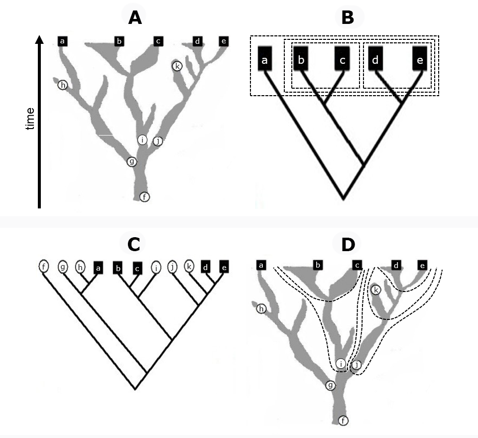
Properties of the Coral
Coral diagrams (Figure 1) can simultaneously present a multitude of features. A branching coral is a rather irregular, bi(multi-)furcating shape (silhouette) placed into a Cartesian coordinate system, with population (group) size (diversity) or morphological difference expressed on the horizontal axis and time measured on the vertical axis. Horizontal cross section of a coral at a given point in time is a partition of life into equivalence classes, and the entire coral may be conceived as a spatiotemporal continuum of these classes. The corals have a tree component because they may be reduced into a (backbone) mathematical tree. This operation is conceivable in the reverse direction: Cladograms with many terminal taxa may be condensed into corals to demonstrate the relative diversity of large clades. Extension to three dimensions, as mentioned above, is also plausible. For visualizing hybridization or other types of relationships between different lineages, interconnections (anastomoses) between branches9 are also allowed (“fan corals”). For more formal definitions, see Podani (2017,2019).
Preparation and Use of Coral Diagrams
Coral BSDs are not a direct outcome of any objective analysis, unlike cladograms, dendrograms, phylogenetic networks, or partitions (nonhierarchical classifications). Rather, corals are drawn by hand to combine analytical results with knowledge from various research fields into a single image. Drawing a coral diagram for the entire life (as in Podani,2019) or for any particular group requires a large amount of information: Cladograms summarizing sister group relationships, morphological cladograms for hypothesizing past ancestor–descendant or sister group relationships between extinct species, divergence times between pairs of taxa based on fossil-calibrated molecular data, paleontological sources on the appearance and extinction of evolutionary lineages, and the number of species of different groups in the past and present. Other information, such as the geographical distribution of taxa and timing of major geological and evolutionary events (mass extinction and emergence of evolutionary novelties, among others) may also be superimposed onto the drawing. The actual realization of a coral involves artistic elements, such as in the design and positioning of branches (the “shape” of phylogeny). Furthermore, since our knowledge on the past is much more limited than that on the present, species richness changes may only be illustrated by extrapolation into the past, which necessarily involves arbitrariness.
Regarding scientific use, coral diagrams serve as a vehicle for simultaneously synthesizing classification, phylogeny, evolutionary relationships, paleontology, geology, and species richness. Very often, corals are no more than models of phylogeny, for example, in comparisons of species “trees” and gene trees. In addition, they are particularly useful summaries of life, or the parts thereof, for educational purposes in textbooks of systematics and evolution as well as in natural history museum displays.
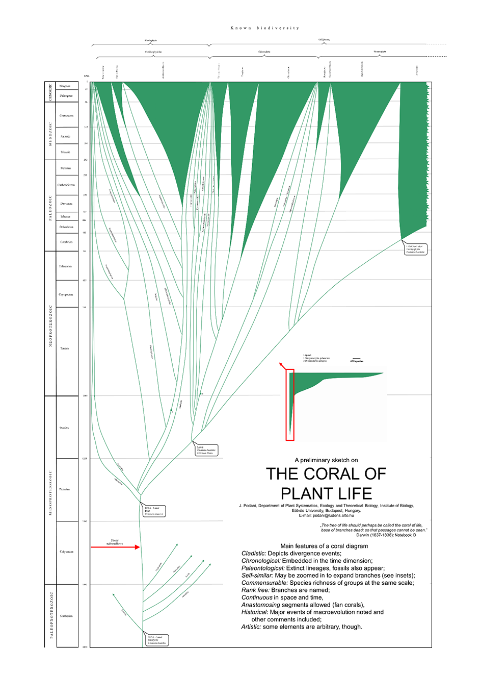
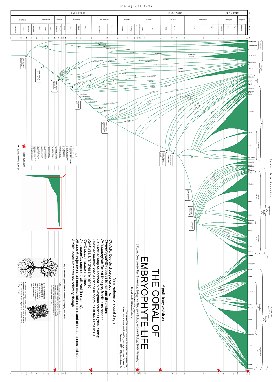
The Coral of Plant Life
In a previous paper (Podani,2019), I have included a preliminary sketch of the Coral of Life for more than two million recent species of prokaryotes and eukaryotes. By zooming out a small part of this is derived the Coral of Plant Life, representing approximately 351,000 recent species as well as many extinct branches and lineages. The general principles and methods in this study are identical to those applied to the entire living world, in addition to some special issues pertaining to plants detailed below.
What are Plants?
Consistent with the current opinion, plants (Plantae; sensu Cavalier-Smith,1981) are photosynthetic organisms whose plastids are of primary endosymbiotic origin.8 This branch on the Coral of Life emerged around 1,450 million years ago (mya), when a nonphotosynthetic unicellular eukaryote engulfed a cyanobacterium, which was then integrated into the host cell as a new organelle – the plastid. This explains both of its newly coined names, the Primoplantae (Palmer et al.,2004) or Archaeplastida (Adl et al.,2005). Many other photosynthetic groups, such as brown algae, diatoms, or dinophytes, also considered plants until recently, are phylogenetically independent from the plant lineages, except that their plastids originated from unicellular red or green algae through secondary or tertiary endosymbiosis (Keeling,2013). The nonphotosynthetic group of fungi, also considered plants for a long time until Whittaker (1969) proposed the five kingdom classification, is even farther away and is phylogenetically much closer to animals than to plants.
Classification and Nomenclature
Since the coral is a historical representation of life, for classificatory purposes, I use historical entities, that is, branches of the coral “detached” at particular time points, especially where bifurcation occurs (Figure 1D). A given branch may correspond to a single species or a collection of two or more, depending on the level of resolution of the coral. For naming coral branches, Linnaean ranks and the associated nomenclature are abandoned and the phylogenetic nomenclature (PhyloCode; http://www.phylocode.org/) is adopted, even though it was originally designed to regulate the naming of clades. As noted by Cellinese et al. (2012) and illustrated in their Figure 1, clades are synchronous entities (i.e., “monophyletic sets of lineage representatives” living at the same time) at terminals of a “tree” (which is in fact a coral because links or edges correspond to lineages in their diagram). A consequence of this definition is that names in the PhyloCode are not meant to designate lineage segments and branches.7 However, the PhyloCode remains much more appropriate for our purposes than the rank-based Linnaean system, because the contents of branches are determined (more precisely, estimated) based on cladograms, some of which are apparently asynchronous (Figure 1). In fact, while deriving the phylogenetic nomenclature of tracheophytes, Cantino et al. (2007) do not insist on synchrony at all but rather describe and name many clades that contain extinct taxa (see their Figure 1, which is an asynchronous cladogram, with both extant and extinct groups as endpoints).
If no such name is found for a group, most often for traditional orders and families (retained in APG I–IV, 1998,2003,2009,2016 and PPG I,2016), a well-known and generally accepted Linnaean name associated with that group is applied to the corresponding branch, as in Podani (2015). Of note, Smith and Brown (2018) followed a similar practice for families and orders. For example, Rosaceae as a branch includes all recent and fossil species classified traditionally in the family in addition to all unknown species that are descendants of the same, unknown ancestor which is also a member of the branch. This practice may be considered as an expansion of the node-based definition of clades (Cantino et al.,2007). If a branch contains a single known species at its end, such as Amborella trichopoda, the branch is named after the genus, Amborella, as the lowest supraspecific rank, while Amborellaceae and Amborellales are deemed redundant and therefore discarded. However, this does not mean at all that the genus rank is accepted here as such and merely indicates the uncertainty whether the branch represents the same single species throughout its length.
The genus poses an insurmountably difficult situation: it is not only a rank but also the first part of the binomen of a given species. That is, classification and nomenclature are not separated at this level of the Linnaean taxonomic hierarchy. Ideally, in a completely phylogenetic, rank-free system (for arguments, counter-arguments, and summary of proposals, see Cellinese et al.,2012, Dayrat et al.,2008, and references therein), species should also be named by uninomials such that no nomenclatural changes would be necessary when the classification changes. However, the binominal nomenclature and genera are deeply rooted in our biological thinking; they have long been used for communication purposes in millions of scientific and popular books, articles, CD-ROMs, videos, and other media and cannot be overwritten or replaced. Keeping the genera would be less of a problem for contemporary organisms, although they cannot be maintained as historical entities without violating the criterion of monophyly. In brief, assume that we have two groups of plants, each with several living species. Both groups are morphologically homogeneous, and the constituting species are much closer to one another than to the members of the other group; therefore, the taxonomist uses two genera, A and B, for their classification and naming. If these genera are sisters in the cladistic sense, then the following question arises: how should their latest common ancestor species be classified and named? If it were added to either A or B and named accordingly, then the genus selected would become paraphyletic; however, if assigned to a third genus, C, this new genus would be immediately paraphyletic and ahistorical. In other words, genera, as most people still treat them, are right at the point where the conflict between the Linnaean and phylogenetic/cladistic thinking is the most striking. The simplest solution is perhaps to retain formally the current binomial names and treat them as two-part “uninomials” for all species (Sundberg & Pleijel,1994) and not to “revise” the names and “rearrange” classifications according to modern cladistic analyses at the “genus level.” Consequently, a species with the binomen Genusa viridis can be considered the ancestor of another species Genusb splendens without violating the monophyly criterion. Of course, I understand that consensus on this suggestion in the scientific community will be difficult to find in the near future.
Clades Approximating Major Branches
Archaeplastida is generally, although not unanimously, considered a monophyletic group (for contrasting views, see Mackiewicz and Gagat,2014). It has three major clades markedly unequal in size, namely the glaucophytes (~20 species), rhodophytes (~7,300 species), and green plants (Viridiplantae, ~343,000 species), while the membership of some other groups (such as Cryptista and Picozoa) is strongly debated. The relative position of these three groups is controversial; the most common view being that glaucophytes are sister to the clade comprising rhodophytes plus green plants, although some recent molecular phylogenetic studies have suggested that rhodophytes are basal (i.e., the smaller sister at the root of the clade; Gawryluk et al.,2019). Since these groups diverged from one another around 1,300 mya, the uncertainty about their branching topology is quite understandable. Here, I keep the more traditional view while placing the origin of these groups close to one another at the root of Archaeplastida to indicate this uncertainty.
Relationships within rhodophytes here are reproduced according to Yang et al. (2016) and Zuljevic et al. (2016). The basal position of Cyanidiales is without doubt, which is then followed by two smaller clades. I retained the conventional notion that Stylonematales is sister to Compsopogonales, although another study including fewer taxa (Muñoz-Gómez et al.,2017) has placed this group as sister to Rhodellophyceae. Both surveys confirm that an overwhelming majority of rhodophytes belong to the monophyletic Eurhodophytina (Bangiales plus Florideophyceae). A recent study identified a new nonphotosynthetic lineage with a relic primary plastid without genome as sister to rhodophytes (Rhodelphis; Gawryluk et al.,2019).
Green plants are divided into two large groups, namely Chlorophyta and the Streptophyta (Leliaert et al.,2012,2016), with two minor branches (Mesostigma and Chlorokybus plus Spirotaenia) as sisters to streptophytes (see also Gitzendanner et al.,2018). This topology is supported by both molecular and cell biological evidence. The branching structure at the base of chlorophytes remains uncertain; therefore, I followed Leliaert et al. (2016) and Sánchez-Baracaldo et al. (2017). Within Streptophyta, the branching sequence of Charophyceae, Coleochaetophyceae, and Zygnematophyceae has been ambiguous for a long time. Most recently, the latter was considered sister to embryophytes (see, e.g., Leliaert et al.,2016 and Ruhfel et al.,2014).
At the base of embryophytes, three clades, namely hornworts, liverworts, and mosses, are each monophyletic with high support, although their relative positions have been uncertain for long. The current view agrees with the conventional one that these together form a clade (see F.-W. Li et al.,2020). While the colloquial term “bryophytes” refers to all three lineages (as in F.-W. Li et al.,2020), the formal name Bryophyta usually designates only one of them – the mosses. To resolve this ambiguity, I suggest the name “Monosporangiophyta” to refer to the entire group (hornworts, liverworts, and mosses). The name emphasizes the major difference between this group, in which a sporophyte bears a single sporangium, and its sister, the Polysporangiophyta, whose sporophytes are branched and produce many sporangia.
All extant members of Polysporangiophyta develop vascular system and comprise the Tracheophyte clade. In this, lycopods (Lycopodiophyta) and euphyllophytes (Euphyllophyta) correspond to the first bifurcation. This arrangement is supported by molecular data as well as an array of morphological differences (Qiu et al.,2006). Euphyllophytes are divided into Monilophyta (i.e., ferns and fern allies; all groups in the traditional Pteridophyta minus lycopods; Kenrick & Crane,1997) and Spermatophyta (the seed plants). For Monilophytes, I have mostly followed PPG I (2016), except that Equisetophyta is shown as sister to the Psilotaceae plus Ophioglossales clade (as in Grewe et al.,2013) to comply with the estimated divergence times (see below). Extant seed plants comprise Acrogymnospermae (gymnosperms) and Angiospermae (flowering plants).
The phylogeny or, more precisely, the cladistics of angiosperms is perhaps the most intensively studied subject in botanical systematics, since Chase et al. (1993) challenged the classical dichotomy between monocots and dicots on molecular basis. As the number of taxa and genes studied increased over the past decades and an increasing number of research groups became involved, the cladogram of angiosperms was refined and became increasingly stabilized (APG I–IV, 1998,2003,2009,2016). Even more up to date is the Angiosperm Phylogeny Website (Stevens,2001), diagrams of which served as the basis for compiling the backbone tree of the coral here. It has long been confirmed that a single species, Amborella trichopoda, is sister to all other angiosperms, followed by Nymphaeales and Austrobaileyales. Moreover, right after the Magnoliales clade separates, there is a major dichotomy between monocots (Monocotyledoneae) and the rest of dicots. In the latter arises the eudicot clade (Eudicotyledoneae) containing over 85% of extant plant species, with superrosids and superasterids as the dominant groups.
Extinct Groups – Extinct Species
The cladistic classification outlined above is based on extant species. They significantly outnumber the fossil ones, and besides, most details of plant phylogeny are “reconstructed” based on information on extant organisms. However, the problem is not only that relatively few extinct plants are known. The fossil records are extremely unbalanced across different groups, depending mostly on biological and geological conditions that determine how the plant material can be preserved. Geological time is another important factor: Plant material is scarce when we reach the older strata. For example, from the Proterozoic (>541 mya), which was the era of important events in archaeplastid evolution and diversification, only a few fossils of rhodophytes (e.g., Bangiomorpha pubescens) and green algae (e.g., Proterocladus antiquus) have been described, and the interpretation of some remnants as plants is sometimes doubtful (Tang et al.,2020). Monosporangiates appear first as fossilized spores; those of liverworts in the Paleozoic (~450 mya) and of hornworts only putatively in the Mesozoic (~140 mya). The first fossil interpreted as a moss (Akdalophyton) was identified from the Late Ordovician (400 mya; Salamon et al.,2018). Regarding more recent ages (up to 66 mya), the number of moss species hardly reaches 70, and the fossil records become richer only in the Cenozoic (Shelton et el.,2015). Protracheophytes (in the Rhynie chert) and tracheophytes are preserved much better and in relatively large numbers from the Silurian through the Mesozoic, offering a wide range of taxa, including many lycopods, sphenopsids, zygopteridalean, and other ferns; progymnosperms; and early seed plants, representing a grade toward extant gymnosperms and angiosperms (“pteridosperms”; Hilton & Bateman,2006), known only as fossils. Most of these do not directly and easily fit into a classification primarily constructed to include extant plants. Extending the synchronous cladogram and redrawing it as a coral by adding fossil taxa are challenging, with the result always burdened by much uncertainty. Cladistic analysis based on morphological characters may be most useful in this work. For supplementing the ancient part of the coral with fossil groups, diagrams in Kenrick and Crane (1997), Hilton and Bateman (2006), Rothwell and Stockey (2008), Crepet and Niklas (2018), Elgorriaga et al. (2018), Cascales-Miñana et al. (2019), and Servais et al. (2019) were used.
The coral offers ample space for illustrating the position of noted representatives of fossil material with small, numbered circles. For example, the oldest multicellular rhodophyte Bangiomorpha pubescens, an important finding for the calibration of early eukaryotic evolution (Gibson et al.,2017), is numbered 1 in Figure 2. Metzgeriothallus sharonae (Hernick et al.,2008), which is the earliest known megafossil (not a spore) of liverworts, is numbered 31 in Figure 3. As we know today, the earliest known angiosperm Montsecchia vidalii (Gomez et al.,2015), an aquatic plant most likely related to the Ceratophyllum clade, is numbered 29 in the same diagram.
In addition to the known and most remarkable fossils with precise stratigraphic dating, the place of hypothetical ancestors of major groups, which represent milestones in evolution, may also be shown in this image. The Coral of Plants in Figure 2 originates at the last eukaryotic common ancestor (LECA; Margulis et al.,2006). As an analogy, I suggest showing the positions of the latest plant common ancestor (LPCA) and the latest embryophytic common ancestor (LEMCA), among others. Further interpretative aid is to indicate the date of major evolutionary events, such as the acquisition of cyanobacteria by a eukaryote at the origin of plant life (red arrow, Figure 2) or the dates of mass extinctions (red stars at the right, Figure 3).
Figure 2
Detail of the Coral of Plant Life, with embryophytes shown in full in Figure 3. High-resolution image is provided as Appendix S2.
Geological Time Scale – Divergence Times
The coral diagram is embedded in a two-dimensional coordinate system with time as the vertical axis. Many illustrations of the Tree of Life (cf. Podani,2019) use a log scale to underweight the past ages, thus leaving relatively more space for illustrating recent events. This scale type is much less intuitive than the linear one when it is to appreciate how much time has passed between two evolutionary events. Therefore, I strongly suggest the use of the linear time scale, as in the Coral of Life. However, the Coral of Plants thus illustrated is unbalanced, because for a small fraction of plants comprising nearly 18,000 extant species (glaucophytes, red algae, green algae), the evolutionary timescale spans ~1,500 million years, whereas for the other species-rich fraction of plants (embryophytes with 333,000 extant species), this scale spans ~540 million years. Therefore, the Coral of Plants is presented here in two parts (Figure 2, Figure 3), with an inset in each to visualize the silhouette in full. On the left side of the figures is shown the geological time scale with eras and periods (Figure 2) as well as epochs (Figure 3), following the current official system of the International Commission on Stratigraphy (Cohen et al.,2013).
Divergence times between sister groups in the cladogram of plants were derived from the internet database Timetree.org (Kumar et al.,2017) by taking the median age for clades for which two or more estimates were available. These estimates are highly variable, since the molecular methods and databases from which cladograms are derived have changed a lot in the past decade. Emergence of new fossils used in the calibration also greatly influences the estimates. For example, for the basal dichotomy of the angiosperm cladogram, between Amborella trichopoda and all other angiosperms, 41 different time estimates have been suggested in the literature (studies between 2002 and 2018), ranging from 99.2 to 279 mya, with a median of 180 mya and estimated value of 181 mya (i.e., in the Jurassic). This range of 179.8 years is only 6 million years shorter than the entire Mesozoic (Triassic, Jurassic, and Cretaceous taken together)! More recently, H.-T. Li et al. (2019) provided confidence intervals for different nodes in plant phylogeny based on 80 genes and 2,881 angiosperm plastomes. For the basal dichotomy, they obtained a range of 266–186 mya and the median of 210 mya, indicating that this event dates back to the late Triassic. This single example succinctly demonstrates the extent of uncertainty involved in estimating the date of past evolutionary events. In some cases, cladogram topologies and time estimates were conflicting, whereas in other situations, the discovery of new fossil material with precise geological timing considerably modified the molecular estimates. Therefore, dating the divergence events as well as the crown clade ages in the entire coral diagram can only be considered putative and is subject to change when new fossils are found and more precise calibration procedures become available.
Species Richness Data
The horizontal axis of the coordinate system is scaled to the number of species. In practice, the total number of extant species determines the number of species corresponding to a given measurement unit (cm or pt). Species richness data for different groups were obtained from Stevens (2001), Christenhusz and Byng (2016), and Guiry and Guiry (2020). In Figure 2, the entire horizontal axis corresponds to 18,000 species plus a small fraction of embryophytes, and one scale unit represents richness of 400 species. In Figure 3, the corresponding values are 333,000 and 1,000, respectively.
The number of fossil species is a completely different matter. As mentioned above, our knowledge on the past is very limited compared with that on the present. This is demonstrated clearly by Niklas et al. (1985) in a summary of the number of plant species described from different geological epochs and ages. Their report was based on approximately 18,000 citations to fossil plant species predominantly from the Northern Hemisphere. From the Middle Devonian, they reported ~45 species, mostly lycopods, zosterophylls, and trimerophytes. The total number of species was raised to 220 in the Carboniferous and to 240 in the Permian. By the Upper Jurassic, this number reached 250, including over 100 conifers. In the Cretaceous, they refer to ~90 pteridophytes. Although these values are obvious underestimates, their conclusions remain valid in general, even though the species list has become longer since then. However, at the scale of the coral, these numbers cannot be shown adequately for technical reasons. In Figure 3, lines are drawn at 2-point width, which corresponds to 125 species, a much higher number than that we know from any group from the Paleozoic, for example. In conclusion, the richness of small groups cannot be shown proportionally. The other difficulty, as I pointed out (Podani,2019), is that for many branches of the coral, fossil data are scarce or unavailable; therefore, the shapes can only be drawn to show gradual diversification, starting from the latest divergence event found for each clade. Since we shall never have complete richness data from the past, the coral will always have a strong heuristic component.
Final Remarks
I consider the Coral of Plants as a preliminary sketch, notwithstanding the fact that it is constructed using large amounts of information derived from many sources. Experts of different taxonomic groups are welcome to refine the details in further editions and revisions of the diagram. In fact, any part of the coral may be redrawn at a refined scale if we have sufficient information on the phylogeny and species richness of selected taxa. Detailed parts will have the same fundamental structural properties as the main diagram – a feature called self-similarity. I have already demonstrated this (Podani,2019) by zooming into the Coral of Life to expand the coral of monocots, the coral of orchids, the coral of lady slipper orchids, and finally, the coral of Cypripedium. In the coral of Cypripedium, the geographical distribution of different branches was also illustrated, showing the possibility to expand the contents of the coral into the direction of biogeography. At this scale of the diagram, even hybridization events could be indicated. Self-similarity may be used extensively if the coral and its zoomed details are incorporated into an online application, in a manner which is technically, albeit not theoretically, similar to the Tree of Life explorer of Rosindell and Harmon (2012).