. Introduction
Gentiana L. (gentian) contains almost 400 species worldwide, whereas approximately 30 species grow in Europe (Xu et al., 2017). Because of their bitter content, they are used in folk medicine to treat the lack of appetite. In addition to the bitter compounds, many xanthones, flavonoids, alkaloids, iridoids and triterpenoids have been reported as active substances in gentian plants (Pan et al., 2016). These compounds can act biologically in various ways, including as hepatoprotective, choleretic, anti-inflammatory, antinociceptive, antiamnesic, antiplatelet, and antiproliferative agents (Mirzaee et al., 2017; Pan et al., 2016).
Literature on gas chromatography (GC) of gentians is scarce. Koshioka et al. (1998) identified endogenous gibberellins in Gentiana triflora Pall. using GC with mass spectrometry (MS) and the Kovats retention indices. Mihailović et al. (2011) analyzed Serbian samples of Gentiana asclepiadea L., highlighting the importance of essential oils and identifying major compounds. Mustafa et al. (2016) compared the volatile profiles of Gentiana lutea L. root materials from wild and cultivated sources. Gas chromatography was also used to identify bitter substances in Gentiana olivieri Griseb. (Azadbakht et al., 2020) as well as for profiling beverages containing the root of G. lutea L. as the bitter ingredient (Biehlmann et al., 2020; Gibitz-Eisath et al., 2022).
No studies have performed comparative analysis of many gentians using GC. The lack of such studies can be attributed to the limitation associated with reliability of such comparisons. The phytochemical composition of plant material can depend on various vegetation factors, such as soil, weather, and light conditions. For instance, a significant correlation between γ-pyrone content and cultivation altitude was reported in Montenegro for G. lutea L. (Balijagić et al., 2012). Gentiopicrin and swertiamarin also varied significantly according to the altitude of Gentiana macrophylla Pall. cultivated in China (Sadia et al., 2020), whereas many active compounds of Gentiana straminea Maxim. varied significantly according to cultivation location in the Tibetan Plateau (Zhou et al., 2021).
These differences can be suppressed by the cultivation of various gentians in the same location, such as in botanical gardens. However, this approach is very difficult in practice, as gentians occur mainly at high altitudes, and their cultivation in the lowlands is simply unsuccessful. A promising alternative is to grow such plants in vitro under optimized conditions (Thiem et al., 2008) and such an approach can provide a high content of the active ingredients (Drobyk et al., 2015a, 2015b). When all plants are grown in the same medium in a conditioned room, the differences in phytochemical composition arise only from differences between species.
These facts encouraged us to analyze a representative set of in vitro cultured gentian species. Our previous research (Gadowski et al., 2022) focused on thin layer chromatography (TLC). This study is a continuation of this research using headspace GC, which is a broad and common technique used to analyze various types of samples (Wang et al., 2008). In the case of plant material, fresh or dried plants can be placed directly in the sample vial, and the gas phase above the sample can be analyzed. Owing to the possibility of sample heating, a large part of biologically active phytochemical constituents can be detected with this method, as they become volatile at high temperatures.
. Material and Methods
. Plant Material
Plant material was obtained from the seeds supplied by various botanical gardens. We obtained whole plants for the separate analysis of roots (K) and shoots (P), as well as calli obtained from the cotyledon (L), hypocotyl (H), and root (R). Previously described methods were followed for the various in vitro procedures used in these experiments (Mikuła et al., 2011; Tomiczak et al., 2015, 2019). Table 1 lists the 72 samples of the 21 species used in this study.
Table 1
List of analyzed samples with their abbreviations. The last letter of the abbreviation indicates the analyzed part or culture: roots (K), shoots (P), and callus obtained from cotyledon (L), hypocotyl (H), and root (R).
Approximately 1.25 g of fresh plant material was weighed accurately for the extraction. Extraction was performed in an ultrasonic bath at a temperature of 35–40 °C for 30 min. For the extraction mixture, we used 25 mL of methanol, acetone, and water in a ratio of 3:1:1. Extraction was performed three times for each sample. The combined extracts were evaporated to dryness by using a vacuum evaporator. The dry residue was dissolved in methanol (5 mL).
. Chromatography
The samples were analyzed using a 7890A gas chromatograph coupled to a triple quadrupole mass spectrometer combined with a 7697A headspace sampler (Agilent Technologies, Palo Alto, CA, USA). Separation was carried out using a chromatographic capillary column HP-5MS ((5%-phenyl)-methylpolysiloxane), 30 m × 0.25 mm i.d., 0.25 µm film thickness) with pure helium (99.9999%; Messer, Chorzów, Poland) as the carrier gas, with a constant flow of 1.0 mL min−1. The mass spectrometer was tuned using perfluorotributylamine to m/z values of 69.0, 264.0, and 502.0. The GC column was operated in the temperature-programmed mode with an initial oven temperature of 40 °C (held for 2 min), ramped to 250 °C at a rate of 15 °C min−1, and held at this temperature for 4 min. The temperatures of the injector, ion source, MS transfer line, and quadrupoles were 250 °C, 230 °C, 300 °C, and 150 °C, respectively. The injections (1 µL) were performed in the split mode with a split ratio of 10:1. The mass detector was operated in the scan mode with standard electron impact conditions (70 eV). To eliminate metastable helium species, helium gas (2.25 mL min−1) was used as the quench gas. The data were collected over a mass-to-charge range of 30 to 500 m/z at a rate of 4 scans s−1. The headspace sampler was connected to the GC system front inlet via a heated fused-silica transfer line. A 1 mL sample loop was employed. The temperatures of the headspace oven, loop, and transfer line were set to 90 °C, 100 °C, and 115 °C, respectively. The injections (sampling time, 0.8 min) were performed in the flow-to-pressure mode (15 psi). The system was operated using the software Agilent MassHunter B.07 (build 7, service pack 2). The extraction of organic compounds from the examined herbal samples was performed using 20 mL headspace vials containing 2 g of dried and ground material. The vials were sealed with a polytetrafluoroethylene-lined septum and an aluminium crimp cap and then conditioned for 20 min at 90 °C. Once equilibrium was reached, the vials were pressurized to 15 psi for 1 min. Chromatograms were recorded for 17 min, starting from the third minute of operation (3–20 min).
. Chemometric Analysis
All data were computed in the GNU R 4.1 computational environment, operated under R Studio (www.r-project.org, www.rstudio.com). The obtained total ion count (TIC) chromatograms were imported from the CSV file, which can be found in each data folder. Average mass spectra of the samples were obtained by converting the entire dataset to MZXML with the ProteoWizard “mzconvert” tool, and subsequently importing to R with the “readMzXmlData” package with a resolution of 0.1 m/z.
. Results
Two matrices with 72 rows (samples) were obtained. The m/z matrix had 4201 columns (mass ranging from 30.0 to 450.0, with steps of 0.1), whereas the TIC matrix had 1201 columns (time points from 4 to 14 min, with steps of 5 s). The principal component analysis results of the concatenated matrix are presented in Figure 1. Figure 2 presents the linear discriminant analysis performed on the first four principal components. The coefficients of the discriminant functions are also illustrated. The features along the mass dimension are presented in Figure 3, and those along the time dimension are presented in Figure 4.
Figure 1
Scores of principal component analysis: (A) PC1 vs. PC2, (B) PC3 vs. PC4. The points and labels are colored according to the tissue type. For an explanation of the labels, see Table 1.
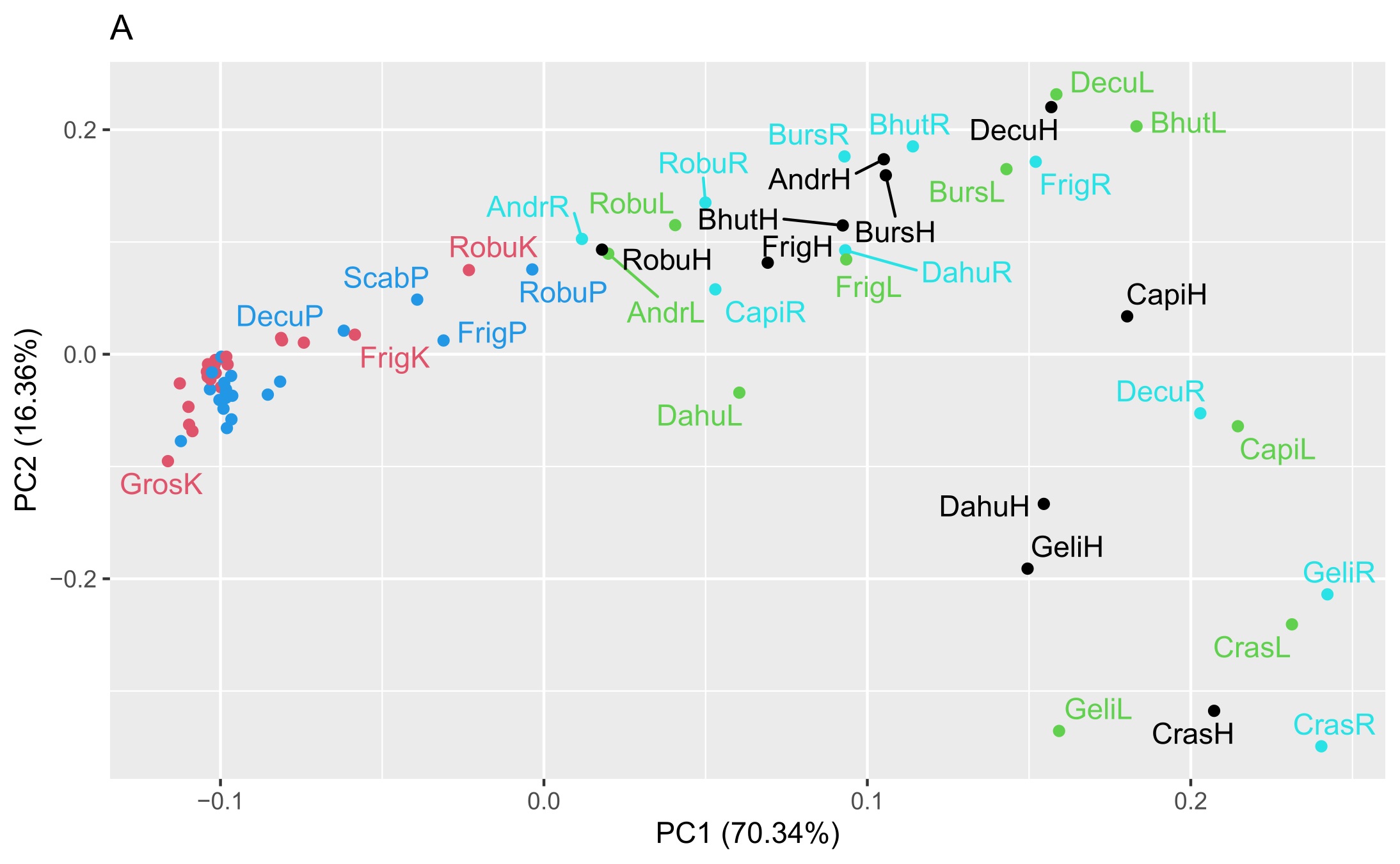
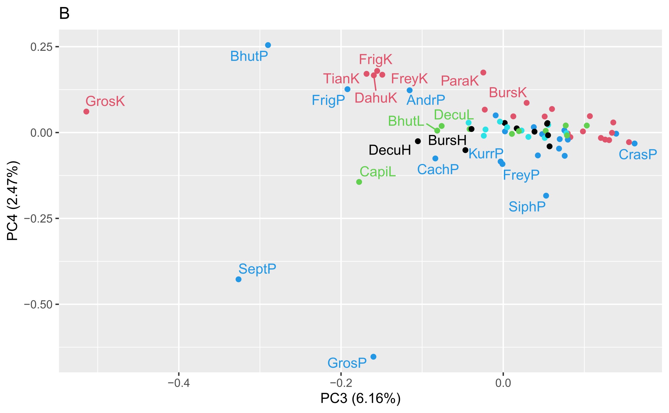
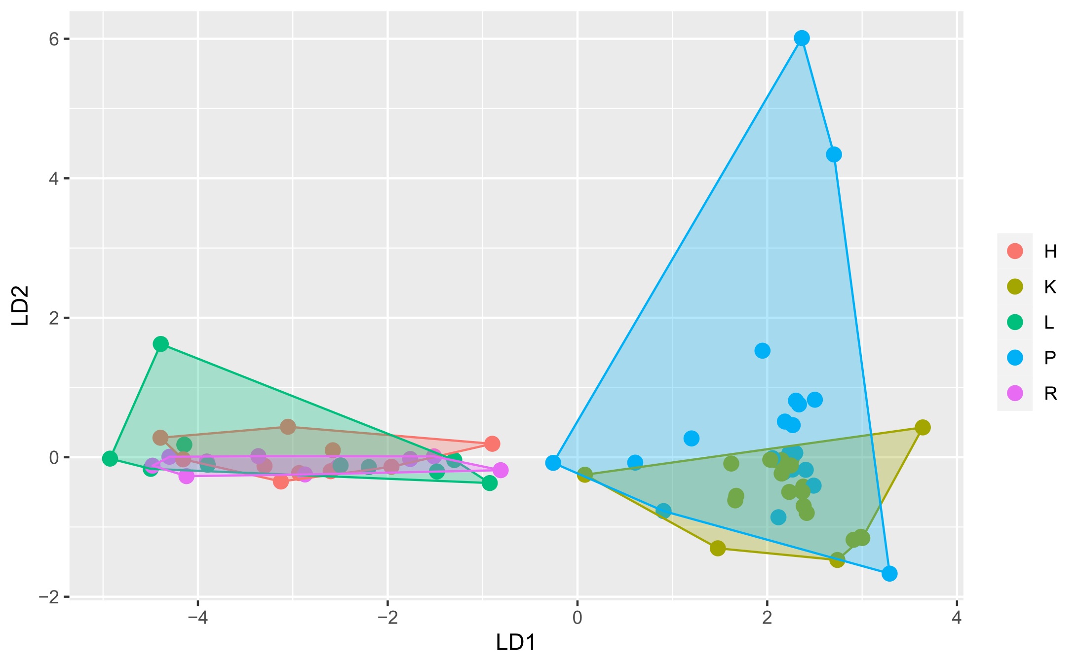
Figure 2
Scores of the principal component–linear discriminant analysis with convex hull polygons grouping tissue types. For an explanation of letters indicating tissues, see the “Plant Material” section.
. Discussion
Initially, we attempted to place fresh plant material directly into the headspace sample vial. However, this method results in very weak chromatograms with unacceptable sensitivity. Therefore, we decided to perform liquid extraction, evaporate the extract, and dissolve it in methanol, similar to the method followed in our previous TLC study (Gadowski et al., 2022). Although there was a risk of loss of volatile compounds, the resulting chromatogram had many more peaks.
We decided to reject mass values below 50.0 before the preprocessing step, as these values caused large variance disturbances in the data analysis. The matrices were concatenated, and each block was scaled separately to the unit variance.
The use of two vectors (the TIC and average MS spectrum vectors) instead of a large matrix was proposed and discussed in our previous paper (Wróbel-Szkolak et al., 2022). Briefly, this approach allows a substantial reduction in the computer resources needed for the computation, as each sample, being a large matrix, can be converted to two small vectors, those of TIC and average mass spectrum. Although it is a lossy compression, this method was demonstrated to separate the main sources of variance regardless of its nature (such as one peak, tailing baseline, and column bleeding with several peaks).
Preliminary analysis of this dataset by principal component analysis (Figure 1) revealed that the four first principal components (PC1–PC4) explained 70.3%, 16.4%, 6.2%, and 2.5% of the variance, and the subsequent components contained only noise or irrelevant information. As shown in Figure 1A, PC1 modelled the difference between the shoot or root cultures (negative values) and callus cultures (positive values). There was no clustering trend along PC2 or PC3 (Figure 1B). A slight tendency to separate the roots (positive values) and shoots (negative values) was also observed along PC4 (Figure 1B).
Because of the discriminative tendency along the PC1 and PC4 axes, one can conclude that the features responsible for cultural differences can be highly complex, and that they are separated from the directions modelling the largest variance. To investigate this phenomenon, we used linear discriminant analysis on the first four principal components. As shown in Figure 2, this method identified the combinations of the first four PCs that best discriminated the culture analyzed: the first discriminant fully separated root or shoot and callus cultures, and the second discriminant represented the difference between shoot (positive) and root (negative) cultures; however, there were several samples that were not separated. The remaining discriminants did not exhibit any discriminative power.
To identify the chromatographic features modelled by these two discriminants, their coefficients (each had four coefficients, assigned to each principal component) were converted to the original multivariate space with matrix multiplication by the loadings of principal component analysis. The resulting matrix can be perceived as the linear discriminant analysis loadings (discriminant coefficients) in the original space.
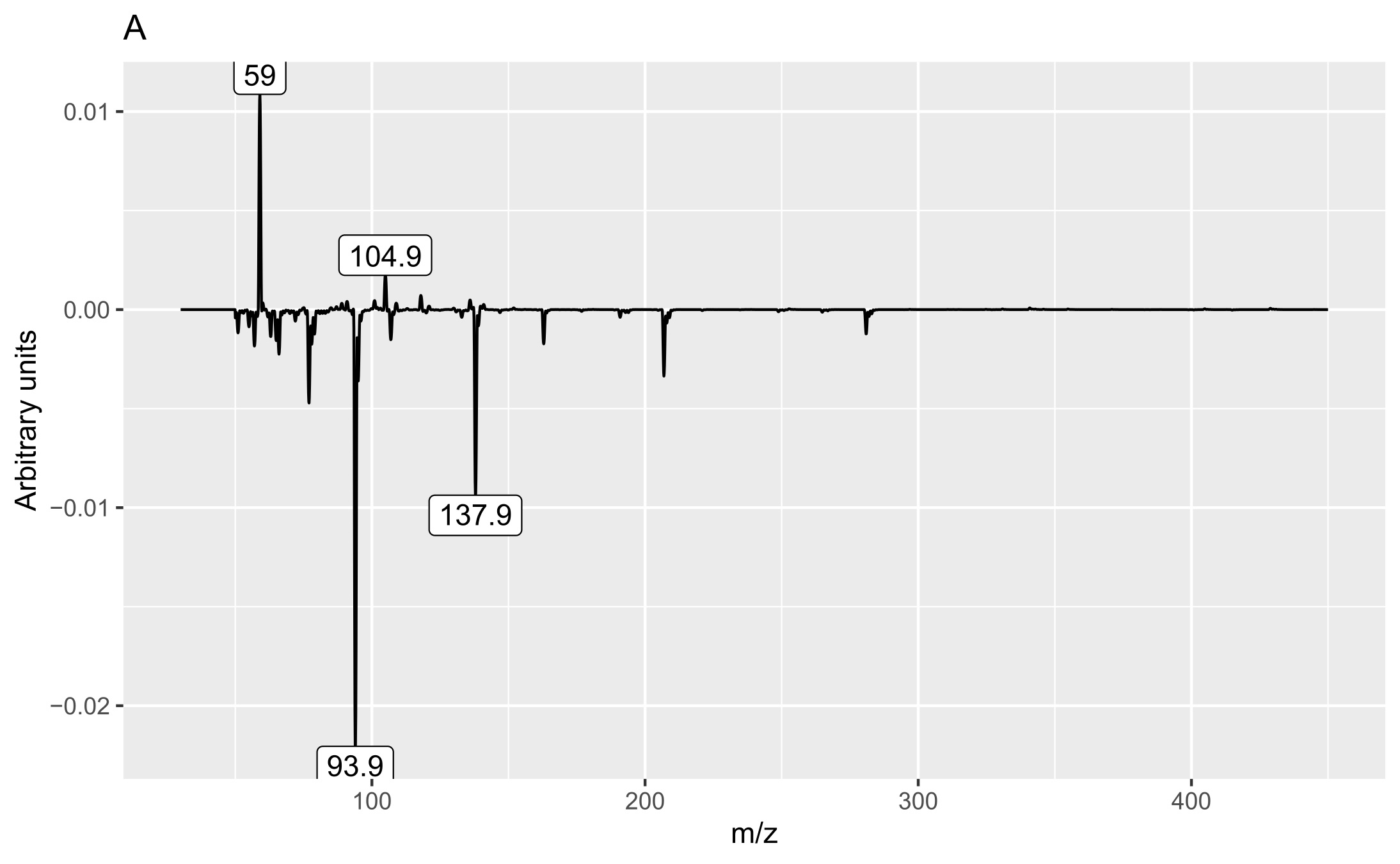
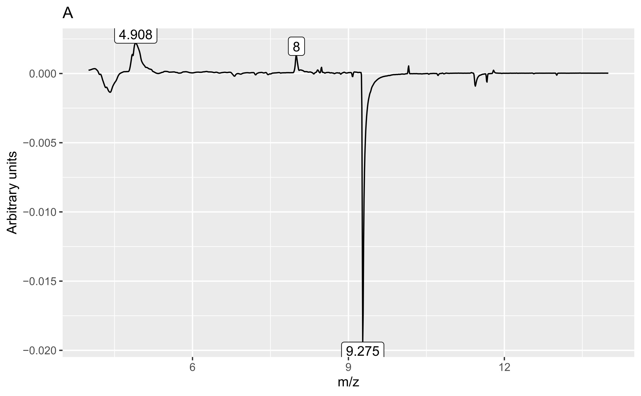
Analysis of the loadings (Figures 3 and 4) revealed that the main feature responsible for the difference between callus and shoot or root cultures (first discriminant) was the presence of a peak with a retention time of 9.275 min (Figure 4A) and mass values of 93.9 and 137.9 (Figure 3A). The peak was present in callus cultures but absent in root or shoot cultures and contained mass and relative abundance values as follows: 93.9, 100%; 137.9, 48.7%; 77, 24.6%; 66, 9.8%; 106.9, 7.6%; and 51, 6.2%. Unfortunately, the identity of the peak could not be determined using the NIST library.
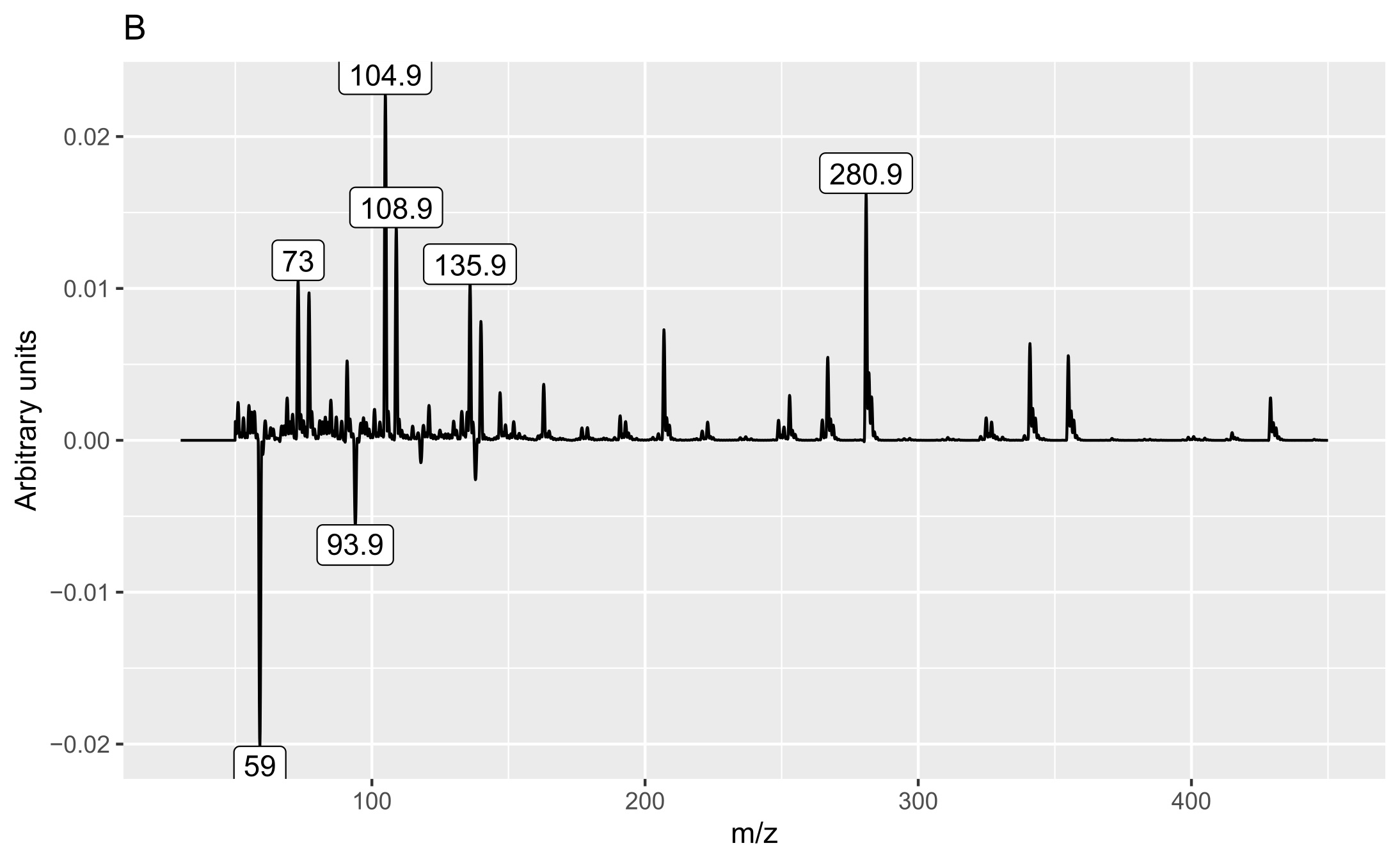
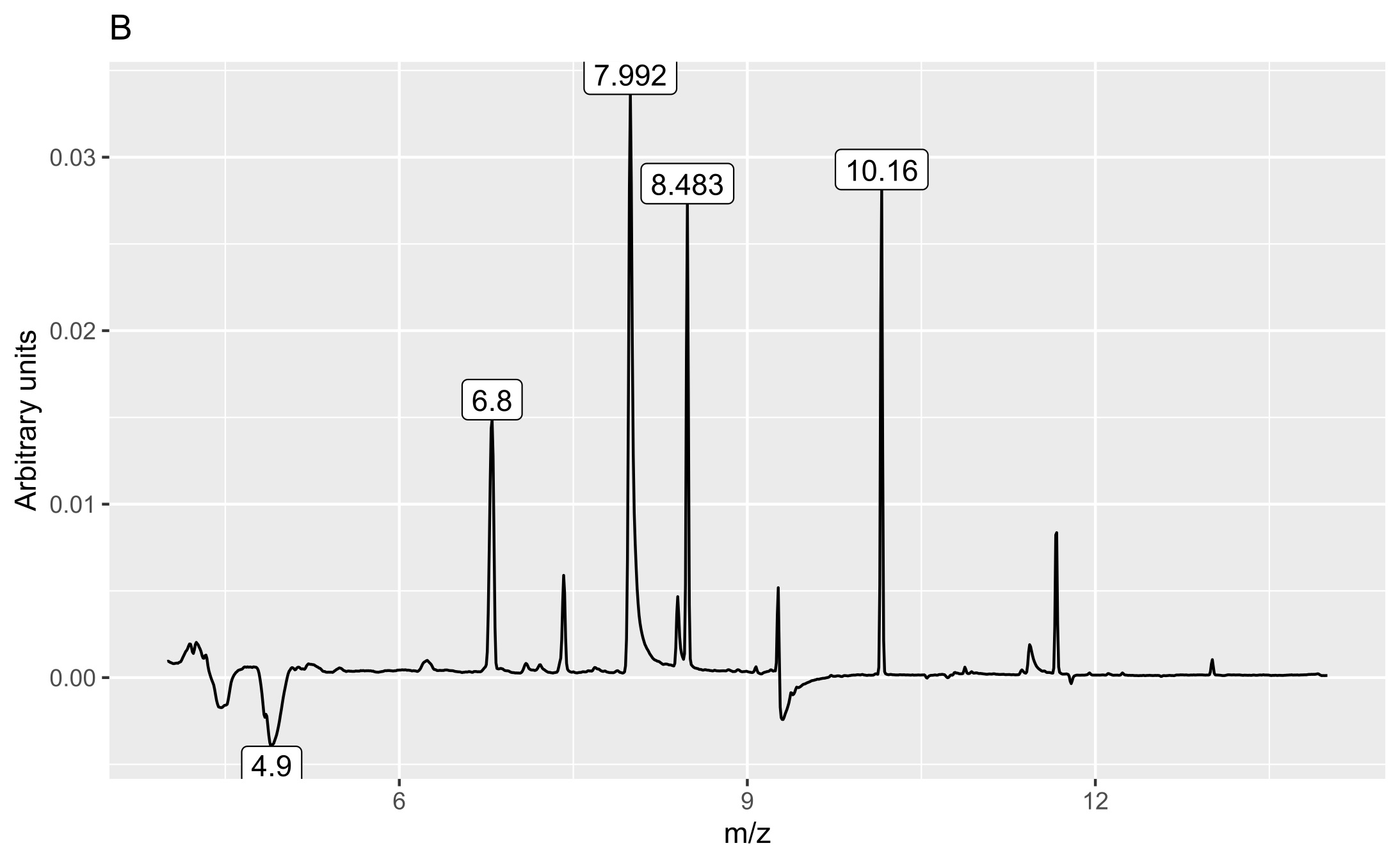
The second discriminant was connected to several peaks (6.8, 7.99, 8.49, and 10.16 min) and mass values: 73, 104.9, 108.9, 135.9, and 280.9. They were more intense in shoot samples than in root samples.
The peak with a retention time of 6.8 min and principal mass of 280.9 was identified as polysiloxane column bleeding. The peak at 7.99 min contained the following mass and relative abundance values: 108.9, 100%; 139.9, 51.7%; 109, 13.4%; 52.9, 7%; 44, 6.5%; 109.1, 5.2%; 73, 5.2%, whereas that at 10.16 min these values were 340.9, 100%; 73, 62.4%; 428.9, 49.9%; 342.9, 23.3%; 341.9, 22.8%; 146.9, 22.7%; 324.9, 21.5%; 430.9, 15.2%; 429.8, 11.4%; 341.3, 9.1%; 341, 7.3%; 72.9, 6.9%; 206.9, 6%; 429.3, 5.5%; 341.2, 5.3%; and 340.8, 5.2%. The last peak with a retention time of 8.49 min contained mass and relative abundance values of 354.9, 100%; 108.9, 14%; 355.9, 7.4%; 355, 6.6%; 42.9, 6.5%; 94.7, 6.4%; 338.9, 6%; 355.3, 5.9%; and 31.1, 5.2%. We could not identify these two substances with the available libraries because we obtained several very different hits with comparative similarity.